MATH2019 Introduction to Scientific Computation
Hello, dear friend, you can consult us at any time if you have any questions, add WeChat: daixieit
MATH2019 Introduction to Scientific Computation
— Coursework 2 (10%) —
Submission deadline: 3pm, Tuesday, 5 Dec 2023
Note: This is currently version 3-2 of the PDF document. (24th November, 2023)
No more new questions will be added anymore. (Just possibly some minor corrections)
This coursework contributes 10% towards the overall grade for the module.
Rules:
• Each student is to submit their own coursework.
• You are allowed to work together and discuss in small groups (2 to 3 people), but you must write your own coursework and program all code by yourself.
• Please be informed of the UoN Academic Misconduct Policy (incl. plagiarism, false authorship, and collusion).
Coursework Aim and Coding Environment:
• In this coursework you will develop Python code related to algorithms that solve nonlinear equations, and you will study some of the algorithms’ behaviour.
• As discussed in the lecture, you should write (and submit) plain Python code (.py), and you are strongly encouraged to use the Spyder IDE (integrated development environment). Hence you should not write IPython Notebooks (.ipynb), and you should not use Jupyter.
How and Where to run Spyder:
• Spyder comes as part of the Anaconda package (recall that Jupyter is also part of Anaconda). Here are three options on how to run Spyder:
(1) You can choose to install Anaconda on you personal device (if not done already).
(2) You can open Anaconda on any University of Nottingham computer.
(3) You can open a UoN Virtual Desktop on your own personal device, which is virtually the same as logging onto a University of Nottingham computer, but through the virtual desktop. The simply open Anaconda. Here is further info on the UoN Virtual Desktop.
• The A18 Computer Room in the Mathematical Sciences building has a number of computers available, as well as desks with dual monitors that you can plug into your own laptop.
Time-tabled Support Sessions (Thursdays 12-1pm, Fridays 5-6pm):
• You can work on the coursework whenever you prefer.
• We especially encourage you to work on it during the (optional) time-tabled drop-in sessions.
Piazza (https://piazza.com/class/llxk0wzpvnpn3):
• You are allowed and certainly encouraged(!) to also ask questions using Piazza to obtain clarification of the coursework questions, as well as general Python queries.
• However, when using Piazza, please ensure that you are not revealing any answers to others. Also, please ensure that you are not directly revealing any code that you wrote. Doing so is considered Academic Misconduct.
• When in doubt, please simply attend a drop-in session to meet with a PGR Teaching Assistant or the Lecturer.
Helpful resources:
• Python 3 Online Documentation – Spyder IDE (integrated development editor) – NumPy User Guide – Matplotlib Quick Start Guide – Moodle: Core Programming 2022-2023 – Moodle: Core Programming 2021-2022 – Moodle: Core Programming 2020-2021
• You are expected to have basic familiarity with Python, in particular: logic and loops, functions, NumPy and matplotlib.pyplot. Note that it will always be assumed that the package numpy is imported as np, and matplotlib.pyplot as plt.
Some Further Advice:
• Write your code as neatly and read-able as possible so that it is easy to follow. Add some comments to your code that indicate what a piece of code does. Frequently run your code to check for (and immediately resolve) mistakes and bugs.
• Coursework Questions with a “? ” are more tedious, but can be safely skipped, as they don’t affect follow-up questions.
Submission Procedure:
• Submission will open approximately a week before the submission deadline.
• To submit, simply upload the requested .py-files on Moodle. (Your submission will be checked for plagiarism using turnitin.)
• Your work will be marked (mostly) automatically: This is done by running your functions and comparing their output against the true results.
Getting Started:
• Download the contents of the “Coursework 2 Pack” folder from Moodle into a single folder. (More files may be added in later weeks.)
• Open Spyder (see instructions above), and if you wish you can watch a basic intro video from the Spyder website (click “Watch video”).
• You can also watch the recording of Lecture 1, second hour, where a brief demonstration was given.
Gaussian elimination without pivoting
(This is a warm up exercise. No marks will be awarded for it. Its solution will appear on Moodle. Further clarification of what you need to do to obtain marks will become clear once more questions are released.)
Suppose that A ∈ Rn×n and that b ∈ Rn . Also suppose that A is such that there exists a unique solution x ∈ Rn to Ax = b and that forward elimination can be per-formed without interchanging any rows or columns to arrive at an augmented matrix to which backward substitution can be applied to find x.
A pseudocode algorithm for performing forward elimination on the matrix M = [ A b ] without interchanging any rows or columns is:
For i = 1, 2, . . . , n − 1 do
For j = i + 1, i + 2, . . . , n do
Set g = mj,i/mi,i
Set mj,i = 0
For k = i + 1, i + 2, . . . , n + 1 do
Set mj,k = mj,k − g ∗ mi,k
End For
End For
End For
The warmup.py file contains an unfinished function with the following first line:
def no_pivoting (A ,b ,n , c ) :
The input A is of type numpy.ndarray with shape (n, n) and represents the square matrix A. The input b is of type numpy.ndarray with shape (n, 1) and represents the column vector b. The input n is of type int and is such that n ≥ 2. The input c is of type int and is such that 1 ≤ c ≤ n − 1. The input c is used to (prematurely) stop the forward elimination algorithm as described below.
Complete the no pivoting function so that the output M is of type numpy.ndarray with shape (n, n + 1) and represents the augmented matrix arrived at by starting from the augmented matrix [ A b ] and performing forward elimination, without interchanging any rows or columns, until all of the entries below the main diagonal in the first c columns are 0.
Note that in the pseudocode algorithm given above, the entries of the matrix M are mi,j for i = 1, 2, . . . , n and j = 1, 2, . . . , n + 1. However, the elements in M (a numpy.ndarray with shape (n, n + 1)) are M[i,j] for i = 0, 1, . . . , n − 1 and j = 0, 1, . . . , n.
The warmup.py file contains an unfinished function with the following first line:
def backward_substitution (M , n ) :
The input M is of type numpy.ndarray with shape (n, n + 1) and represents an aug-mented matrix of the form [ U v ] where U ∈ R n×n is an upper triangular matrix with all entries on its main diagonal being nonzero and v ∈ R n . The input n is of type int and is such that n ≥ 2.
Complete the backward substitution function so that the output x is of type numpy.ndarray with shape (n, 1) and represents the solution x to Ux = v.
Hint: See Lecture 4 Slides, Algorithm 6.1, Steps 8 and 9.
The warmup.py file also contains a finished function with the following first line:
def no_pivoting_solve (A ,b , n ) :
A test that you can perform on your no pivoting and backward substitution functions is to run the main warmup.py file and check that what is printed is:
[[ 1. -5. 1. 7.]
[ 0. 50. 10. -64.]
[ 0. 35. -6. -31.]]
[[ 1. -5. 1. 7. ]
[ 0. 50. 10. -64. ]
[ 0. 0. -13. 13.8]]
[[ 2.72307692]
[ -1.06769231]
[ -1.06153846]]
(The below has been added on 17 Nov 2023.)
Gaussian elimination with complete pivoting
Suppose that A ∈ R n×n , that det(A) = 0 and that b ∈ R n .
1 Given matrix V ∈ R n×n with components vj,k, a pseudocode algorithm for finding integers p and q such that the integer q is the smallest integer for which 1 ≤ p ≤ n, 1 ≤ q ≤ n and
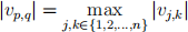 (1)
(1)
and, for this q, the integer p is the smallest integer for which 1 ≤ p ≤ n and (1) holds, is the following:
Set m = 0
Set p = 1
Set q = 1
For k = 1, 2, . . . , n do
For j = 1, 2, . . . , n do
If |vj,k| > m
Set m = |vj,k|
Set p = j
Set q = k
End If
End For
End For
The systemsolvers.py file contains an unfinished function with the following first line:
def find_max (M ,n , i ) :
The input M is of type numpy.ndarray with shape (n, n + 1). The input n is of type int and is such that n ≥ 2. The input i is of type int and is such that 0 ≤ i ≤ n − 2.
Complete the find max function so that the outputs p and q are both of type int and are such that the int q is the smallest integer for which i ≤ p ≤ n − 1, i ≤ q ≤ n − 1 and
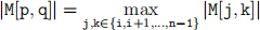 (2)
(2)
and, for this q, the int p is the smallest integer for which i ≤ p ≤ n − 1 and (2) holds.
A test that you can perform on your find max function is to run the Question 1 cell of the main.py file and check that what is printed is:
1
0
Assessment
When submitting your coursework, you will only be asked to upload your systemsolvers.py file.
Marks can be obtained for your find max function for generating the required out-put, for certain sets of inputs for {M, n, i}. The correctness of the following will be checked:
• The type of the outputs;
• The values of the outputs.
Note that in marking your work, different sets of inputs may be used. [10 / 40]
2 The systemsolvers.py file contains an unfinished function with the following first line:
def complete_pivoting (A ,b ,n , c ) :
The input A is of type numpy.ndarray with shape (n, n) and represents the square matrix A. The input b is of type numpy.ndarray with shape (n, 1) and represents the column vector b. The input n is of type int and is such that n ≥ 2. The input c is of type int and is such that 1 ≤ c ≤ n − 1. The input c is used to (prematurely) stop the forward elimination with complete pivoting algorithm; see details below.
Complete the complete pivoting function so that:
– The output M is of type numpy.ndarray with shape (n, n + 1) and repre-sents the augmented matrix arrived at by starting from the augmented matrix [ A b ] and performing forward elimination with complete pivoting (as de-scribed in the Linear Systems: Direct Methods II slides) until all of the entries below the main diagonal in the first c columns are 0.
– The output s is of type numpy.ndarray and has shape (n,) and is what is arrived at by starting with s=np.arange(n) and interchanging s[j] and s[k] whenever column j and k of the augmented matrix are interchanged.
The complete pivoting function should call the find max function.
Hint: M[[j,k],:]=M[[k,j],:] can be used to interchange row j and row k of M.
Hint: M[:,[j,k]]=M[:,[k,j]] can be used to interchange column j and col-umn k of M.
Hint: s[[j,k]]=s[[k,j]] can be used to interchange s[j] and s[k].
A test that you can perform on your complete pivoting function is to run the Question 2 cell of the main.py file and check that what is printed is:
[[20. 0. 10. 6. ]
[ 0. -5. 0.5 6.7]
[ 0. 10. 5.5 4.3]]
[2 1 0]
[[20. 0. 10. 6. ]
[ 0. 10. 5.5 4.3 ]
[ 0. 0. 3.25 8.85]]
[2 1 0]
Assessment
When submitting your coursework, you will only be asked to upload your systemsolvers.py file.
Marks can be obtained for your complete pivoting function for generating the required output, for certain sets of inputs for {A, b, n, c}. The correctness of the following will be checked:
• The type of the outputs;
• The shape of the outputs;
• The values of the outputs.
Note that in marking your work, different sets of inputs may be used. [10 / 40]
3 The systemsolvers.py file contains an unfinished function with the following first line:
def complete_solve (A ,b , n ) :
The input A is of type numpy.ndarray with shape (n, n) and represents the square matrix A. The input b is of type numpy.ndarray with shape (n, 1) and represents the column vector b. The input n is of type int and is such that n ≥ 2. Complete the complete solve function so that the output x is of type numpy.ndarray with shape (n, 1), and represents the solution x ∈ R n to Ax = b computed using Gaussian elimination with complete pivoting followed by appropriate use of what is returned from the backward substitution func-tion. Note that a completed version of the backward substitution function is in the warmup solution.py file that is imported in systemsolvers.py. A test that you can perform on your complete solve function is to run the Ques-tion 3 cell of the main.py file and check that what is printed is:
[[ 2.72307692]
[ -1.06769231]
[ -1.06153846]]
Assessment
When submitting your coursework, you will only be asked to upload your
systemsolvers.py file.
Marks can be obtained for your complete solve function for generating the re-quired output, for certain sets of inputs for {A, b, n}. The correctness of the following will be checked:
• The type of the output;
• The shape of the output;
• The values of the output.
Note that in marking your work, different sets of inputs may be used. [4 / 40]
(The below has been added on 24 Nov 2023.)
Weighted Jacobi method
Suppose that A ∈ R n×n , that det(A) = 0, that all of the entries on the main diagonal of A are nonzero and that b ∈ R n . Let x ∈ R n be the solution to Ax = b.
Starting from an initial approximation x (0) ∈ R n , the approximation to x obtained after k iterations of the weighted Jacobi method (which is not studied in the lectures) is the vector x (k) ∈ R n with entries

where the weight w is an appropriate positive number. Note that if w = 1 then this method is the Jacobi method.
Note that the vector form of the above weighted method is:
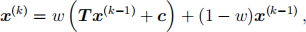
where T = D−1 [L + U] and c = D−1b, and A = D − L − U is the decomposition of A as discussed in Lecture 7.
4 The systemsolvers.py file has been updated to include an unfinished function with the following first line:
def weighted_Jacobi (A ,b ,n , x0 ,w , N ) :
The input A is of type numpy.ndarray with shape (n, n) and represents the square matrix A. The input b is of type numpy.ndarray with shape (n, 1) and represents the column vector b. The input n is of type int and is such that n ≥ 2. The input x0 is of type numpy.ndarray with shape (n, 1) and represents the ini-tial approximation x (0). The input w is of type float and represents the weight w. The input N is of type int and is the number of iterations to be performed. Complete the weighted Jacobi function so that the output x approx is of type numpy.ndarray with shape (n, N + 1) and is such that, for j = 0, 1, . . . , n − 1, x_approx[j,0] = x (0)j+1 and x approx[j, k] = x (k)j+1 for k = 1, 2, . . . , N.
Hint: You can choose to implement the element-based form or the vector form of the method. When doing the vector form, the following functions could be useful: np.dot, np.tril, np.triu, np.diag, np.linalg.inv, np.matmul or the ’@’ operator for matrix multiplication (see Lecture 7 Slides and Notes, as well as the end of Lecture 7 recording for a coding demonstration.)
A test that you can perform on your weighted Jacobi function is to run the Question 4 cell of the updated main.py file and check that what is printed is:
[[ 0. 0.33333333 0.14285714]
[ 0. 0. -0.35714286]
[ 0. 0.57142857 0.42857143]]
Assessment
When submitting your coursework, you will only be asked to upload your systemsolvers.py file.
Marks can be obtained for your weighted Jacobi function for generating the re-quired output, for certain sets of inputs for {A, b, n, x0, w, N}. The correctness of the following will be checked:
• The type of the output;
• The shape of the output;
• The values of the output.
Note that in marking your work, different sets of inputs may be used. [10 / 40]
5 The systemsolvers.py file has been updated to include an unfinished function with the following first line:
def weighted_Jacobi_plot (A ,b ,n , x0 , weights ,M , N ) :
The input A is of type numpy.ndarray with shape (n, n) and represents the square matrix A. The input b is of type numpy.ndarray with shape (n, 1) and represents the column vector b. The input n is of type int and is such that n ≥ 2. The input x0 is of type numpy.ndarray with shape (n, 1) and represents the ini-tial approximation x (0). The input weights is of type numpy.ndarray with shape (M,) and is an array of values for the weight w. The input M is of type int and is such that M ≥ 1. The input N is of type int and is the number of iterations to be performed.
Complete the weighted Jacobi plot function so that the output fig is of type matplotlib.figure.Figure and is a figure (with a single pair of axes) on which is plotted k x − x (k)k ∞ for k = 0, 1, . . . , N with the weight w = weights[i] for i = 0, 1, . . . , M − 1. This figure should have a legend with M entries from which the values of w and which plotted points a particular value corresponds to can be seen.
The approximations x(k) to x should be computed by calling the weighted Jacobi function. The solution x to Ax = b should be computed by calling the no pivoting solve function. You may assume that the matrix A is such that forward elimination can be performed without interchanging any rows or columns to arrive at an augmented matrix to which backward substitution can be applied to find x. Note that a completed version of the no pivoting solve func-tion is in the warmup solution.py file that is imported in systemsolvers.py.
Hint: To calculate the l∞ norm of a vector represented by a one-dimensional numpy.ndarray u, one can use np.linalg.norm(u,np.inf).
Hint: If v is of type numpy.ndarray with shape (n, m) and p is a nonnegative int less than m then w[:,p] is of type numpy.ndarray with shape (n,) not (n, 1). A test that you can perform on your weighted Jacobi plot function is to run the Question 5 cell of the updated main.py file.
Assessment
When submitting your coursework, you will only be asked to upload your systemsolvers.py file.
Marks can be obtained for your weighted Jacobi plot function for generating the required output, for certain sets of inputs for {A, b, n, x0, weights, M, N}. The correctness of the following will be checked:
• The points plotted;
• The legend.
Note that in marking your work, different sets of inputs may be used. [6 / 40]
Finished!
2023-12-04