EE 5410 Signal Processing MATLAB Exercise 2
Hello, dear friend, you can consult us at any time if you have any questions, add WeChat: daixieit
EE 5410 Signal Processing
MATLAB Exercise 2
Sinusoidal Interference Cancellation
Intended Learning Outcomes:
On completion of this MATLAB exercise, you should be able to
. Analyze discrete-time signals in the frequency domain
. Design and implement a digital filter for suppressing a sinusoidal interference
Deliverable:
. Each student is required to submit a hardcopy answer sheet which contains only answers to the questions in this manual on or before 7 November 2018.
Background:
A typical application area for least squares filter is interference cancelling. Here, the task is to remove a noise or interference signal with the use of an external reference and its block diagram is shown in Figure 1.
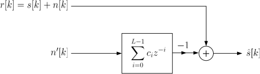
Figure 1: Digital filter for removing an interference
Interference cancelling principle is applicable in cases where there is a signal s[k] embedded in an interference n[k] , together with a reference source of the interference n' [k] . The problem of interference suppression is formulated as follows. Given
r[k] = s[k] + n[k ] and n' [k], k = 0,1, … , N − 1
The task is to recover s[k]. The n[k] and n' [k] are correlated in the sense that n[k] can be modelled as a linear combination of n' [k] :
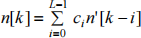
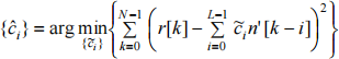
where { ci } are unknown. Based on the technique of least squares filtering [1], the { ci } are estimated as:
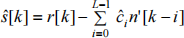
The recovered signal is then calculated as
In telecommunication, a typical application example of interference cancelling is echo cancellation where r[k] contains both the near-end and far-end talker signals while n' [k] is a reference source of the far-end talker signal [2]. Furthermore, in biomedical engineering, a well-known example is in electrocardiogram (ECG) recording where r[k] is an ECG signal corrupted by a 50 Hz power line interference while n' [k] is another 50 Hz signal with different amplitude and phase [3].
Procedure:
1. Download the file “one2nine.txt” at [4]. This file contains the waveform of the numbers “ 1” to “9” and the sampling frequency is 22000 Hz. Try the following MATLAB code
load one2nine.txt
soundsc (one2nine, 22000)
Examine the operation of the commands. Change the number “22000” to “10000” and “40000”. What do you hear for the three cases? Briefly explain the differences.
2. Download the file “message.txt” at [4]. This file contains the waveform of a voice message embedded in a sinusoid with frequency of 300 Hz, and the sampling frequency is 22000 Hz. Construct a least squares filter to recover the speech using the following steps:
(a) Try the following MATLAB code
load message.txt
soundsc (message, 22000)
What do you hear? Can you hear the speech?
(b) Try the following MATLAB code to observe the spectrum of message:
[freq_resp,freq_index]=freqz(message,1,50000,22000); plot(freq_index,abs(freq_resp))
You will see the magnitude plot of the Fourier transform for message versus frequency in Hz. The dominant frequency component of message corresponds to the peak of the magnitude spectrum. Write down the dominant frequency with the use of the command max. For more information, try help freqz and help max.
![]() (c) Since the interference is a sinusoid, it should be of the form:
(c) Since the interference is a sinusoid, it should be of the form:
n(t ) = A cos( ωt + φ)
where ω = 600π while the amplitude A and the phase φ are unknown. After sampling, the discrete-time interference signal is:
n[k] = A cos( ωkTs + φ)
where Ts = 1/ 22000 . From trigonometric identities, n[k] can be written as:
n[k] = A cos(φ)cos(ωkTs ) − Asin(φ)sin(ωkTs )
= αn'1 [k] + βn'2 [k]
where n'1 [k] = cos( ωkTs ) and n'2 [k] = sin( ωkTs ) are known which can be considered as reference sources for n[k] while α = A cos(φ) and β = − Asin(φ) are the unknown weights to be determined. The least squares estimates for α and β are obtained from:
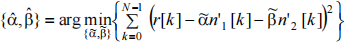
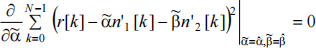
where r[k] corresponds to message. That is, ![]() and β(ˆ) are solved via
and β(ˆ) are solved via
differentiating the least squares cost function with respect to ![]()
![]() then setting the resultant expressions to zero:
then setting the resultant expressions to zero:
and
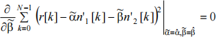
Solve the above two equations. Then write down the estimates of the unknown weights. Note that the summation starts from k=0 . Use length(message) to determine the appropriate signal length, that is, the value of N.
(d) After obtaining  and
and  , write MATLAB code to construct the recovered
speech according to
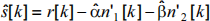
Determine the speech content.
References:
[1] S.D.Stearns and D.R.Hush, Digital Signal Processing with Examples in MATLAB, CRC Press, 2011
[2] S.Haykin, Adaptive Filter Theory, Pearson, 2014
[3] B.Widrow and S.D.Stearns, Adaptive Signal Processing, Prentice Hall, 1985 [4] http://www.ee.cityu.edu.hk/~hcso/ee5410.html
2023-11-25
Sinusoidal Interference Cancellation