CS 335 - Fall 2023: Assignment 3
Hello, dear friend, you can consult us at any time if you have any questions, add WeChat: daixieit
CS 335 - Fall 2023: Assignment 3
Due: Friday November 17, 2023, 11:59pm
Submit all components of your solutions (written/analytical work, code/scripts/notebooks, igures, plots, etc.) to CrowdMark in PDF form in the section for each question.
You must also separately submit a single zip ile containing any and all code/notebooks/scripts you write to the DropBox on LEARN in runnable format (that is, the iles in the zip should be of type .ipynb).
For full marks, you must show your work and adequately explain your logic!
1. (6 marks) Floating Point Basics
(a) (2 marks) Suppose that on a given base-10 loating point system of the form considered in class, the number 23 and the next representable loating point number larger than 23 are separated by 10-3. What is the number of digits, t, in this system?
(b) (2 marks) Using what you found above, what is the spacing between 5 and the next larger representable number in the same loating point system?
(c) (2 marks) Suppose you are now given the fact that the range for the exponent is given by L = —4 and U = 6 in the system above. What is the largest magnitude negative number
 (1)
(1)
2. (8 marks) Efects of Cancellation
We saw in class that adding two numbers of similar magnitude and opposing sign has the potential to cause large relative errors under loating point – this efect is known as catastrophic cancellation, since cancellation of the leading digits causes a disastrous loss of precision. In some cases, however, this efect can be avoided by rearranging the arithmetic expression to be computed.
The roots of a quadratic equation, ax2 + bx + c = 0, are given by

when a ≠ 0.
(a) (3 marks) Consider performing arithmetic in a loating point number system with β = 10, t = 5, L = — 10, U = 10 with truncation. Using the above formulas, you are to simulate by hand (with the aid of a calculator) the computation of the roots of the following quadratic equation
0.2x2 + 14.2x + 1.67 = 0, (2)
under this loating point system. (Obey the usual order of operations.) The true roots of the given quadratic, correct to ive signiicant digits, are —0.11780 and —70.882. What is the relative error of each of your computed roots, x1 and x2 ?
![]()
![]() (b) (2 marks) A cancellation problem arises when applying the above formulae for any quadratic equation having the property that
(b) (2 marks) A cancellation problem arises when applying the above formulae for any quadratic equation having the property that

When this property holds, if b > 0 then the quadratic formula for x1 will exhibit cancella- tion, while if b < 0 then x2 will exhibit cancellation. We will try to circumvent this problem by reformulating our expression. Show that the following formula for x1 ,
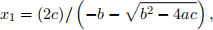
is mathematically equivalent to the usual one given at the start of the question (i.e., as- suming you are working with real numbers rather than loating point numbers.) Hint: Rationalize the denominator of this expression.
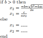
(c) (1 mark) The formula for x2 can be manipulated similarly. Deduce a better algorithm for calculating the roots of a quadratic equation (which avoids cancellation errors), and present it in the form below (i.e., illing in the blanks for the x1 and x2 expressions).
Algorithm R.
(d) (2 marks) Redo the calculation of the roots of equation (2) by applying Algorithm R using the same loating point number system. Compute the relative error of the computed roots and compare against your results from part (a). What do you observe?
3. (8 marks) Floating Point Error Analysis
Show that if x,y, z are already oating point numbers in some loating point system F , the relative error of the loating point calculation (x 一 y) 发 z with respect to the true value of (x 一 y)/z is less than or equal to 2E + E2 (where E is machine epsilon for the FP system F) assuming no overlow/underlow errors occurs.
The symbols 一 and 发 here represent loating point subtraction and division, respectively. Just like we saw for addition in class, they satisfy a 一 b = fl(a 一 b) and a 发 b = fl(a/b), for loating point inputs a and b.
4. (6 marks) Convergence of Fixed Point Iteration
Consider a ixed point iteration:
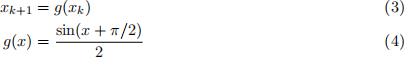
Will this iteration converge for any x 2 [0, π/2]? Justify your answer by considering all the conditions of a convergence theorem.
![]() 5. (16 marks) Root inding methods
5. (16 marks) Root inding methods
In this question you will implement each of the four root inding algorithms discussed in class in a Jupyter/Python notebook. The function prototypes are as follows:
. Bisection method.
def bisection(f, a, b, tol, maxiter):
% This function computes a root of f in the interval [a, b] % using the bisection method .
. Secant method.
def secant(f, a, b, tol, maxiter):
% This function computes a root of f using the secant method % with initial guesses x_{-1} = a, x0 = b .
. Newton’s method.
def newton(f, fprime, x0, tol, maxiter):
% This function computes a root of f using the Newton’s method % with initial guess x0 . fprime should be the derivative of f .
. Fixed point iteration.
def fixedpoint(g, x0, tol, maxiter):
% This function computes a fixed point of g using fixed point % iteration with initial guess x0 .
For each of these functions, the output should be a vector:
x = [x1 , x2 , . . . , xn],
where xk is the approximate solution found after k iterations. The stopping criterion is when either jxn - xn-1 j < tol or the number of iteration exceeds the maximum, maxiter. You will also need to deine the functions f, fprime, g according to the problem to be solved, below. (Note that Python allows you to pass functions as inputs to other functions, as implied by the function deinitions above.)
Find the root (x* = p3) of the following equation:
x2 - 3 = 0, x 2 [0.5, 3.5]
using your four root inding functions with tol=1e-10 and maxiter=100. For the bisection and secant methods, use [a,b]=[0.5,3.5]. For Newton and ixed point iteration, use x0=0.5. You will need to determine a g(x) function such that the ixed point iteration converges. There are multiple valid choices here. (Do not use the g(x) that corresponds to Newton’s method.)
Next, using the root-inding methods above, write code that, for each of the methods, computes the errors of approximations, ek = jx k - x* j, and generates a simple text-format table like the following:
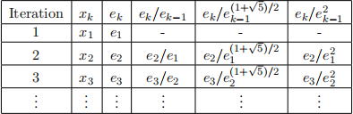
Print the x, e, and various ratio values in scientiic notation. A straightforward way to perform this type of formatting is using the print command, such as in the following (generic) example:
print("Row %d First Number: %0.7f Second Number: %0.7e" % (3, 1.73648392e-8, 1.73648392e-8))
which prints
Row 3 First Number: 0.0000000 Second Number: 1.7364839e-08
The %d is used to indicate an integer. %0.7f and %0.7e are used to display loating point numbers in standard and scientiic notation, respectively, with the integer 7 here indicating the number of digits desired after the decimal. You can also use ’nt’ to insert tabs rather than spaces, such as print("Word1ntWord2"), which may help in aligning text columns. For the last 3 column headers, you can use the simpler titles ’ratio1’, ’ratio2’, and ’ratio3’ in your code, rather than the mathematical expressions shown in the table above.
Using these tables, determine and state the order of convergence for each of the methods. Provide a brief text explanation of how you arrived at your answers.
6. (10 marks) Warrant Pricing
A warrant is a call option which gives the holder the right to pay the strike price and receive shares. In the case of a warrant, the shares are issued by the company, and hence there is a share dilution efect.
Let
K = strike
T = expiry Time
σ = volatility
r = risk free rate
M = number of warrants outstanding
N = number of original shares outstanding S0 = share price
C(S0, K, r, T, σ) = value of a European call option.
Then the price of a warrant, denoted by W , is given by
 (5)
(5)
This is a nonlinear equation for the warrant value.
(a) Write a Jupyter/Python notebook to solve equation (5) based on the data in Table 1. Use a ixed point iteration scheme. Use the provided function blsprice (which calculates the
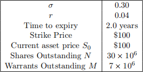
Table 1: Option parameters for Q6.
analytical Black-Scholes price) to evaluate C(S0, K, r, T, σ). If Wk is the kth iterate, stop the iteration when

Use W0 = 0. Let the residual Rk (which measures how far our equation is from being satisied) at step k be deined by
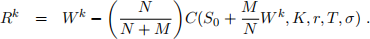
Produce (programmatically) a simple text table of Wk and Rk versus the step number k.
(b) In the same Jupyter notebook, write additional code to solve the warrant pricing problem, this time using Newton’s method. Let Wk be the kth iterate. Let W0 = 0. Use the same stopping criteria as in equation (6). Again, produce a table of Wk and Rk versus k. The provided function blsdelta might be useful, since it provides the derivative of the blsprice function (i.e., option price) with respect to the stock price.
(Side note: blsprice and blsdelta are written to mimic the corresponding MATLAB functions of the same names – thus the MATLAB documentation provides an expanded description, if you are curious.)
2023-11-19