Hello, dear friend, you can consult us at any time if you have any questions, add WeChat: daixieit

Math 4315 Advanced Scientific Computing

Project 1: Iterative Linear Solvers

What to Submit

Please submit your report (in pdf format) with your Matlab routines/scripts as an appendix (see the sample report I uploaded on Canvas). This report must present the results in a logical, readable manner. Deductions and conclusions must be clearly presented and a brief discussion of the problems must be given. Since this is a research report, you will need to

1. present things in complete sentences and paragraphs, not in itemized point format;

2. include Matlab plots/results to support your deductions; and

3. provide a brief introduction on the overall project, tying the different problems together. For example, for this project a short intro can be “… will be exploring iterative linear solvers for the analysis of a diffusive process. The computational bottleneck in the computer simulation is in the solution of large linear systems that arise in the discrete model. In this project, we will …”

The presentation will have a weight on the overall grade of your project.

THE REPORT SHOULD BE ONLY 5-10 PAGES LONG. PLEASE START THIS EARLY. IT WILL TAKE LONGER THAN A FEW HOURS TO DO.

Program Style

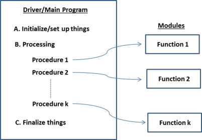
I also would like you to write your codes in a structured, module style. Module programming allows re-use of software that you have already developed and thoroughly tested. It also leads to clean structured codes. Below is a diagram that illustrates the design of a structured and module code. The driver or main program sets up the problem, calls several software modules to perform the overall task, and then finalizes things (e.g., post-process or print/graph the results).

The modules can consist of newly written codes and old codes.

Finally, present your own work. Copying, plagiarism, and fabrication of results will result in discipline.

We will be consider a diffusive process in an infinitesimally thin domain of length L, which we can take to be the line segment [0, L]. The problem may represent the diffusion of heat or some species in the domain.

The mathematical formulation for our model is given by the equations

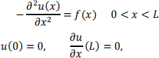
where u(x) is, say, the temperature at location x, and the second-order partial derivative term models the diffusion of the temperature in the domain. The second equation describes two conditions applied at the left and right boundaries (temperature of 0 at the left end and no temperature loss at the right end, i.e. the flux of temperature is 0 at the right end). IT IS NOT NECESSARY FOR YOU TO KNOW HOW ALL THIS IS DERIVED AND TO ANALYZE THIS SYSTEM. Rather, we will solve this numerically, leading to a computer simulation of this application. Here is the numerical approximation:

Let the [0,L] be divided up into (n+1) equally-spaced points spaced out by Δx=L/n, i.e. {x=0, ∆x, 2∆x,…,n∆x =L}. We can simulate the diffusion by solving the following sequence of linear systems:

Au=b

where A is the n-by-n matrix

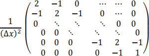
the solution u is an approximation to the temperature at the spatial nodes x=∆x, 2∆x,…,n∆x, i. e.

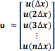
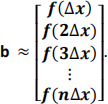
and

Problem 1

Write a matlab routine that generates the matrix A. This function should take in arguments (n, ∆x) and return the matrix A. To get you started, the function should have the handle

function [A]= generate_matrix(n, ∆x)

Test your code for L=1, n+1=11, and print out the matrix. This matrix is of the size 10x10. Please make sure your routine is correct since it will be used in the other parts of this project.

Problem 2,

We will assume that the forcing is f(x) = sin 5πx.

(i) Generate b for this forcing, taking L=1 and n+1=201. Using your routine in Problem 1 to generate A, solve the corresponding linear system using matlab’s backslash solver: i.e. u= A\b. Include a plot of this solution, and save it for later parts of this problem.

(ii) Implement SOR for solving an nxn linear solver. The input arguments to your function should be n, A, b, initial approximation w0 the SOR parameter w, and the number of iterations, and the output should be the approximate solution w to the linear system:

function [w]= SOR(n, A, b, w0, w, niterations)

With n+1= 201, initial approximation 0, and w = 1, apply 3000 iterations of SOR to obtain the approximation w. Plot the residual

r= b – Aw

and the error

e= u- w

on the same plot. Repeat the same process but for w = 1.25. Compare the results for the two different parameter choices.

(iii) Using the better parameter that gave a faster convergence rate, solve the system for n+1=51. Note that because the size of the systems is 4 times smaller, it requires less computation. Does the approximation have the same profile as the solution u. How can you use this fact for improving the efficiency for the n+1=201 case? (Hint: the initial approximation for SOR affects the efficiency of the computation.)

Your driver should have the following structure