ECON 1100: Intermediate Economics Assignment #6
Hello, dear friend, you can consult us at any time if you have any questions, add WeChat: daixieit
ECON 1100: Intermediate Economics
Assignment #6
Due 10/26/2023 by 9:30 AM
Answer the following questions clearly and completely. Be sure to show your work - we need to be able to see how you arrived at your answers so that we can understand your thought process and give full (partial credit if warranted). Be sure to upload your assignment to Gradescope before the deadline. You are welcome and encouraged to work in groups as long as the work you hand in is your own! Do not hesitate to stop by office hours if you have any questions or merely wish to talk through any aspect of the problems. Work hard and good luck!
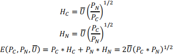
1. Andrew is a deeply committed lover of croissants. Assume his preferences are Cobb-Douglas over croissants (denoted by D on the x-axis) and a numeraire good (note: we use the notion of a numeraire good to represent spending on all other consumption goods – in this example, that means everything other than croissants – its price is normalized such that PN = $1). Assuming Andrew’s utility function is given by 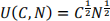 and his income is $64 a year, his Marshallian demand for croissants will be
  . The expenditure
minimization problem yields his compensated (Hicksian) demand for croissants, his compensated (Hicksian)
demand for the numeraire good, and his expenditure function:
a. You’ve been hired by a government official considering a proposed piece of legislation that would increase the price of croissants from $1 to $4 while leaving incomes unchanged. Find the original level of utility
Andrew achieved before the price increase, then compute the Compensating Variation for this price
increase, that is, the minimum amount that Andrew would need to be paid so that he’s no worse off after the price for a box of croissants rises to $4.
b. Draw a rough graph of the Marshallian demand and show the loss of Consumer Surplus that would be
associated with this price increase? Set up the integral that you would use to calculate the loss (no need to actually solve for the area).
c. Now redraw your graph from part (b) and add the compensated demand function for boxes of croissants.
Denote both CV and ∆CS on the graph Identify the difference between CV and ∆CS and clearly label it.
d. What factor causes the divergence between CV and ∆CS to be large or small? Is the divergence between the
two significant in this situation? Support your answer with, at most, two sentences and the numerical values
of the elasticity version of the Slutsky equation (ε = ε * − ξθ).
2. In the following, we are going to use the microeconomic theory we have developed in class to explore the short run implications of the rise in the price of gasoline in 2022 due to various factors, including the war in Ukraine. We can use the “constant elasticity” demand function, Qg = ΦPε y ξ , as a framework for representing the
demand for gasoline. The reason it is named as such is that the exponents for the price of gasoline (P) and
income (y), denote the price elasticity of demand (ε ) and income elasticity of demand (ξ) for all levels of each variable.
a. Use the formula for price elasticity of demand to calculate the price elasticity of demand to show that it equals the parameter ε. Note that you would receive an analogous result if you did this for income elasticity of demand.
b. Use the following estimated values to “calibrate” the constant elasticity demand function, that is, use
algebra to solve for a value for the parameter Φ (phi) based on average annual consumption, average price per gallon, and median US income. Once you are done calibrating, you should be able to write the demand function with numerical values for everything but Q) , P, and Y. Everything you need can be
found in the following real world data that is easily collected by searching the web for relevant economic studies:

Note: we are just looking for a reasonable approximation of short run gasoline demand here. If it was
important to be more precise, we would use data to estimate the demand for gasoline without some of the assumption we are implicitly making here.
c. Using the calibrated demand function you found in part (b), set up the integral that gives the change in consumer surplus when the price of gasoline rises from $3.44 to $4.70 a gallon. Evaluate that integral (your answer will be a function of Y). Please round decimals to the thousandths.
d. We can use the previous results to better understand how the impact of this gas price increase will vary across households with different income levels. Construct a table that has 2 rows that correspond to the following average household income levels: $50,000 and $100,000. You should include the following
columns in your table: average annual household gasoline demand when gasoline costs $3.44, the
percentage of the household annual income spent on gasoline, the loss in consumer surplus due to the price of gasoline rising to $4.70, and the loss of consumer surplus divided by income. Calculate the
values of each cell in your table.
e. Given your table in part (d), how does the impact of the price increase vary over the four income levels examined? Is this the impact of this regressive, that is, does the percentage of income spent by
consumers decrease as income increases.
f. For which income level does the change in consumer surplus the come closest to correctly estimating our preferred measure of welfare loss (compensating variation)? In no more than two sentences, use the Slutsky equation to justify your answer.
2023-10-24