Exam 2 review – STAT 1000/1100
Hello, dear friend, you can consult us at any time if you have any questions, add WeChat: daixieit
Exam 2 review - STAT 1000/1100
Regression
Problem 1:
An elderly individual has a fractured hip and is facing surgery to repair it. The orthopedic surgeon explains the risks to the patient. Infection occurs in 2% of such operations, the repair fails in 10%, and both infection and failure together in1.5%. (Use a Venn Diagram to model this problem.)
What is the probability that the operation succeeds and is free from infection?
a.0.785
b. 0.80
c.0.895
d. 0.81
e. 0.865
problem 2
One of the common tests for tuberculosis (TB) is a skin test where a substance is injected into a subject’s armand we see if a rash develops in a few days. The test is relatively accurate, but in a few cases a rash might be detected even when the subject does not have TB (afalse positive) or the rash may not be seen even when the subject has TB (afalse negative). The probability of a false positive is approximately 0.05 and the probability of a false negative is approximately 0.01. In the U.S. only about 4 in 10,000 people have TB (an incidence rate of 0.0004). Model this with a tree diagram.
Calculate the overall probability of a Positive Test result.
a.0.050376
b.0.9904
c.0.015374
d.0.52
e.0.003322
Problem 3:
What is the theoretical probability of rolling a sum of 10, 11 or 12 on these two 8-sided dice? Hint:
Consider all the possible equally likely outcomes in the sample space.
a.
0.28125
b.
0.19
c.
0.375
d.
0.2375
e.
0.171875
Problem 3:
We would like to explore the relationship between unemployment and the education rates, using the data for 11 states. Let X variable be the percentage of people who attained a Bachelor Degree (Bachelor Degree %), and let Y variable be the ‘Unemployment Rate”
|
STATE |
Bachelor Degree (%) |
Unemployment Rate (%) |
|
Vermont |
36 |
2.9 |
|
Colorado |
38.1 |
3.3 |
|
Utah |
31.1 |
3.8 |
|
Minnesota |
33.7 |
3.3 |
|
Kansas |
31 |
3.5 |
|
Montana |
29.5 |
4.1 |
|
Michigan |
26.9 |
4.7 |
|
New Jersey |
36.8 |
4.7 |
|
Ohio |
26.1 |
4.7 |
|
Nevada |
23 |
4.9 |
|
West Virginia |
19.2 |
5.4 |
Enter the “Bachelor Degree (%)” data into L1 and “Unemployment Rate (%)” data into L2
i. Fit a linear model to this data and store the equation in Y1. Store the predictions in
L3 and the Residuals in L4. What is the resulting equation?
Calculator Steps :
STAT ![]() CALC
CALC ![]() LinReg(a+bx)
LinReg(a+bx) ![]() XList: L1 ; YList: L2 ; Store ReqEq*: Y1
XList: L1 ; YList: L2 ; Store ReqEq*: Y1 ![]() Calculate
Calculate
*to store in Y1, do this: VARS ![]() Y-VARS
Y-VARS ![]() FUNCTION
FUNCTION ![]() Y1 to store
Y1 to store
predicted values: “L3=” ![]() VARS
VARS ![]() Y-VARS
Y-VARS ![]() FUNCTION
FUNCTION ![]() Y1
Y1 ![]() ”Y1(L1)”
”Y1(L1)”
a.) yˆ = 12.117 - 0.3735x
b.) yˆ = 7.2947 - 0.1054x
c.) yˆ = 1.5498 – 1.6175x
d.) yˆ = 20.785 - 0.1076x
ii. How much of the variation in state unemployment rates can be explained when we use Bachelor Degree % as the predictor in our linear model?
a.) 77.3%
b.) 10.5%
c.) 59.9%
d.) 68%
e.) 97.5%
iii. The state of West Virginia has the lowest percentage of people who completed a
Bachelor Degree. What is our predicted unemployment rate, and what is the value of the residual for this state?
a.) yˆ = 4.0%, Residual = 0.21%
b.) yˆ = 30.6%, Residual = 2.96%
c.) yˆ = 4.54%, Residual = 0.16%
d.) yˆ = 5.27%, Residual = 0.13%
iv. Using a calculator, generate a scatter plot of Bachelor Degree % (your X value) versus RESIDUALS (we stored them in L4). Do you see one unusually large residual?
Calculator Steps:
2nd ![]() STAT PLOT
STAT PLOT ![]() ON
ON ![]() TYPE (upper left)
TYPE (upper left) ![]() Xlist: L1, Ylist: L4
Xlist: L1, Ylist: L4 ![]() ZOOM
ZOOM ![]() 9
9
Which of the two statements below correctly describes this unusual value? (use “trace”)
a. Predicted Unemployment rate in New Jersey is much higher than the actual unemployment rate b. Predicted Unemployment rate in New Jersey is much lower than the actual unemployment rate
c. Predicted Unemployment rate in Ohio is much higher than the actual unemployment rate d. Predicted Unemployment rate in Ohio is much lower than the actual unemployment rate
Problem 4:
The concentration (in milligrams per liter) of a medication in a patient’s blood as time passes is given by the data in the following table:
|
Time (hours) |
Concentration (mg/l) |
|
0 |
0 |
|
0.5 |
78.1 |
|
1 |
99.8 |
|
1.5 |
84.4 |
|
2 |
50.1 |
|
2.5 |
15.6 |
i. Fit a quadratic model to this data with your calculator (X: Hours and Y:
Concentration). What are the coefficients, and R-Square of your quadratic model?
a.) yˆ = - .0053x2 – 254.21x + 2059, R-square = .949
b.) yˆ = .0134x2 – 2567x + 11921, R-square = .841
c.) yˆ = - 56.214x2 + 139.31x + 9.35, R-square = .9218
d.) yˆ = 0.000478x2 – 1.82202x + 1737.34, R-square = .9775
ii. Using your calculator to generate predictions (store them in L3) and the residuals (L4). Create a scatter plot: Hours(L1) vs Residuals(L4). Which of the following describes the largest residual?
a.) Time: 0, y: 0 mg/l, yˆ : 9.35 mg/l, Residual: -9.35 mg/l
b.) Time: .5, y: 78.1 mg/l, yˆ : 64.953 mg/l, Residual: 13.147 mg/l
c.) Time: .5, y: 64.953 mg/l, yˆ : 78.1 mg/l, Residual: 13.147mg/l
d.) Time: 1, y: 99.8 mg/l, yˆ : 92.449 mg/l, Residual: 7.3514 mg/l
iii. What is the predicted concentration of medicine in the blood after 2.25 hours have passed?
Hint: plugin 2.25 for X into the equation you stored in Y1
Problem 5 (Teen Birth Rate vs Poverty Level):
This dataset of size n = 51 are for the 50 states and the District of Columbia in the United States. The variables are x = year 2002 birthrate per 1000 females 15 to 17 years old andy = poverty rate, which is the percent of the state’s population living in households with incomes below the federally defined poverty level.
Regression Analysis: Brth15to17 versus PovPct
The regression equation is
PovPct = 4.46 + 0.3883 Brth15to17
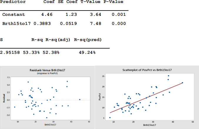
. How much of the variation in poverty rates can be explained by state teen birthrate?
a.) 20.2%
b.) 53.33%
c.) 52.38%
d.) 0.5%
ii. Connecticut in this data had poverty rate of 9.7, and teen birthrate of 14.1.
What is the predicted poverty rate and the residual for Connecticut?
a.) yˆ = 9.93%, Residual = - 0.23%
b.) yˆ = 8.13%, Residual = 1.57%
c.) yˆ = 10.93%, Residual = - 1.23%
d.) yˆ = 7.66%, Residual = 2.04%
iii. What do the residual plot and the R-sq value tell you about the linear model that was created for this data?
a.) The linear trend in the Residual plot indicates that the linear model was a correct model for the data; however, teen birth rates are not good predictors of poverty rates.
b.) The lack of pattern in the Residual plot indicates that the linear model was an incorrect
model for the data and the R-Sq value tells us that teen birth rates are not good predictors of poverty rates.
c.) The lack of pattern in the Residual plot indicates that the linear model was a correct model for the data; however, teen birthrates may not be the best
predictors of poverty rates.
d.) The linear trend in the Residual plot indicates that the linear model was a correct model for the data and the R-Sq value supports that claim.
e.) The lack of pattern in the Residual plot indicates that the linear model was a correct
model for the data and the R-Sq value indicates a strong predictive relationship between x andy.
Problem 6:
Data for total New England Old Navy daily sales and New England March temperatures (F0) was used in Minitab to run linear regression. The following regression equation was generated: yˆ = 23.2 + 1.4x, where x = “degrees in Fahrenheit” andy = “dollar amount in thousands per day”
Which statement best interprets this regression equation:
a.) Average daily sales decrease by $1,400 per one degree(F0) increase in temperature. b.) Average daily sales increase by $14,000 per one degree(F0) increase in temperature.
c.) Average daily sales increase by $1,400 per one degree(F0) increase in temperature. d.) Average daily sales increase by $(1,400+23,200) per one degree(F0) increase in temperature.
Problem 7:
Below is a scatterplot of the weight (lbs) of various cars vs. their Mileage(mpg)
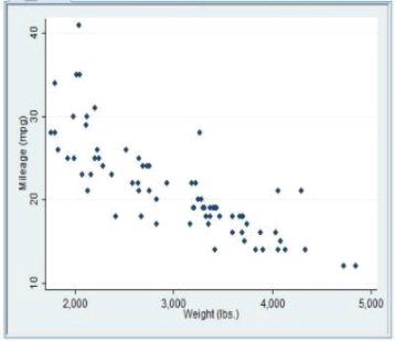
A plausible value for the correlation between Weight(lbs) and Mileage(mpg) could be:
a.) +0.75
b.) - 0.75
c.) +1.4
d.) - 0.1
Problem 8:
A sociologist conducted a study to determine the relationship between years of education,x, and
annual income, y, (in thousands of dollars). From the data, the following statistics were calculated:
![]() = 13.5 Sx = 14.8
= 13.5 Sx = 14.8 ![]() = 57.286 Sy = 29.426 T = 0.93
= 57.286 Sy = 29.426 T = 0.93
i. Use the following equations to create the regression equation for x: years of education and y: annual income
b =T (sy/Sx) and a =![]() −b
−b![]()
y-hat = 32.31 + 1.85 x
2023-10-19