MATH3070 Assignment: Size spectrum modelling
Hello, dear friend, you can consult us at any time if you have any questions, add WeChat: daixieit
MATH3070 Assignment: Size spectrum modelling
This assignment is based on the ZooMSS (Zooplankton Model of Size Spectra) we are
describing in class and using in tutorials. Its formulation is detailed in Heneghan et al. (2020) – see the MATH3070 Blackboard site under Learning Resources/Size spectrum modelling -
Anthony/References + Extra material/.
In this assignment, you will conduct a sensitivity analysis, obtain outputs, and interpret your answers. A sensitivity analysis is a study of how the inputs of a model affect its outputs – in essence, which are the most and least important inputs to the model output. You can learn a lot about a model by conducting a sensitivity analysis. We will conduct a simple sensitivity analysis on a selection of model parameters by varying one parameter at a time while keeping all others constant.
To answer the following questions, run the simulations then use the outputs and your understanding from the equations in the lectures to explain changes in zooplankton and fish biomass. To make it easier to compare outputs from different simulations, there is a csv output file with all the parameters included in the simulation, together with its results. See the following code near the end of setup_RUN_NAME_MATH3070.R. What does this code do?
df <- data.frame(Groups, Abundance = Sspecies, Biomass = WWspecies,
TrophicLevel = TL, CarbonBiomass = C)
write.csv(x = df, file = paste0("Outputs", jobname, ".csv"))
For your assignment answers, you will want to use a combination of the graphs and values for objects in setup_RUN_NAME_MATH3070.R. Note that the variables Sspecies (Abundance), WWspecies (Wet weight), TL (Trophic level) and C (Carbon biomass) all are vectors 12 long, representing the 2 microzooplankton (flagellates and ciliates), 7 main zooplankton groups (larvaceans, omnivorous copepods, carnivorous copepods, euphausiids, chaetognaths, salps, jellyfish), and 3 fish groups (small, medium and large). Their order is the same as in the Species variable in Test_Groups.csv. Also note that the variables Ssize (Abundance) and WWsize (Wet weight) are both vectors 178 long, with each element representing the size classes in the model. The size classes are ordered from smallest to largest.
To help interpret your outputs, please report the wet weight biomass for total zooplankton and total fish (you will need to sum the required elements in WWspecies – the elements are ordered the same as in TestGroups.csv). In your answers, you can also use output from the plots provided, with ggBiomassSizeSpec (ggplot of the Unnormalised Biomass Size Spectrum) and ggBiomassTS (ggplot of biomass of the functional groups over time) being the most useful.
The base case simulation
All simulations will be run in comparison to the base case simulation with parameter values provided in TestGroups.csv. If you think you might have changed the default values, download another copy from Github: https://github.com/MathMarEcol/ZoopModelSizeSpectra.
For this assignment, you will only need to run the program setup_RUN_NAME_MATH3070.R – it calls all other functions needed. To run the sensitivity analysis on a parameter, make sure you are either modifying the TestGroups.csv file or modify the respective variables in the code after reading the file.
For the sensitivity analyses in the assignment questions, use a sea surface temperature (sst) of 15°C and a Chlorophyll-a concentration (chlo) of 0.2 mg.m-3, close to the global mean for
each variable. You will need to modify the enviro_data object. So, in
setup_RUN_NAME_MATH3070.R, you should set:
enviro_data <- fZooMSS_CalculatePhytoParam(data.frame(cellID = 1,
sst = 15,
chlo = 0.2,
dt = 0.01))
For the sensitivity analyses, change the parameter for all the main zooplankton groups (larvaceans, omnivorous copepods, carnivorous copepods, euphausiids, chaetognaths, salps, jellyfish), and keep all others (flagellates, ciliate, small fish, medium fish, large fish) unchanged.
Questions
Note that questions marked * are part of the assignment (i.e., 7 questions). The other questions can be attempted and answers will be provided, but they are not part of the assignment questions.
*1. Run the base case scenario. Describe the outputs. You will be able to use these outputs to compare with the sensitivity analyses and projections below.
Sensitivity analysis: How does changing the search volume change the model output?
The search volume is the volume of water that an animal can search per unit time to ingest food. The search volume is an allometric relationship, with a coefficient (y from lectures and SearchCoef in TestGroups.csv) and exponent (“ from lectures and SearchExp in TestGroups.csv).
*2. The default value for the coefficient of the search volume is 640. Run simulations changing the search volume coefficient to 480 and then 800 for all zooplankton groups. What happens to zooplankton and fish, and the size spectrum and how does biomass change through time. Explain what is happening.
3. The default value for the search volume exponent is 0.8. Change this to 0.7 and then 0.9. What happens to zooplankton and fish and why? When interpreting what happens, note that the weights for zooplankton are <1.
4. Which parameter do you think we would need to know more precisely in the model? Explain your answer.
Sensitivity analysis: How do the Predator Prey Mass Ratios change the model output?
The Predator Prey Mass Ratios (PPMRs, called β in lectures and PPMR in TestGroups.csv) is the relative biomasses of the predator and their preferred prey. Changing PPMR in the model is a bit more challenging than other parameters because the PPMR of some groups changes with body size, rather than remaining constant as an organism grows. This is reflected in TestGroups.csv by the NA for PPMR, and the PPMRscale parameter, which includes the non- linear scaling with body size. To set the PPMR to be constant for each group across its body size, change the PPMR value in TestGroups.csv from NA to any particular value, and change the PPMRscale to NA (see below).
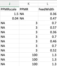
*5. The lowest PPMR for zooplankton is about 3. So, let’s see what happens if we set the PPMR of all zooplankton groups to 3. Describe the outputs. To run this simulation, the relevant columns in your TestGroups.csv should look like this:
*6. A high PPMR for zooplankton is 1,000,000 (they get even higher though!). Set the PPMRs for all zooplankton groups to 1,000,000. What happens and why? Comment on the stability of the system
*7. How does PPMR generally impact the system. How does the PPMR change the slope of the size spectrum?
Sensitivity analysis: How does the carbon content of the zooplankton change the model output?
The carbon content (called Carbon in TestGroups.csv and ‘ in the lectures) is the proportion of body mass that is carbon and reflects the nutritional value of food. For example, jellyfish have a carbon content of 0.005 of their mass because they are mainly water. They can thus be heavy (lots of water), but they are not very nutritious (not much carbon).
8. Set the carbon content for all zooplankton groups to be that of jellyfish. What happens and why?
9. Set the carbon content for all zooplankton groups to be that of the crustacean groups (i.e. 0.12). What happens? Interpret your answer.
Projections: How might climate change affect marine ecosystems, especially fish?
To answer this question, we will not conduct a sensitivity analysis, but instead make projections for the future. You will now be changing the sst and chlo columns in the enviro_data object.
But before you do, make sure you change the TestGroups.csv back to its default values. You can always redownload it from GitHub if needed.
*10. Under a high emissions scenario in 2100, global mean sea surface temperature is likely to increase by about 3°C, depending on the Earth System Model considered. Set the temperature for the model to 3°C above the current global mean temperature we have been using. Run a simulation with the default parameter values in TestGroups.csv. How does global warming impact the marine ecosystem in ZooMSS? Why?
*11. Warming of the ocean surface layer increases the stratification in the ocean, decreases nutrients in surface waters, and leads to declines in phytoplankton (chlorophyll-a). Under a high emissions future scenario, chlorophyll-a is projected to decline by 25% in many ocean regions. How does the impact of climate change on declining chlorophyll-a affect the marine ecosystem modelled in ZooMSS? Why? Is warming or the decline in chlorophyll-a likely to be more important for future fisheries?
12. Finally, run a simulation with the temperature and chlorophyll-a changes together, and see what happens. Interpret your answer. What could this mean for fisheries globally and human livelihoods?
2023-10-16