Hello, dear friend, you can consult us at any time if you have any questions, add WeChat: daixieit

The University of Melbourne

1 Learning Outcomes

2 The Story...

Traffic congestion detection and analysis aims to detect regions of a road network where traffic speed is slow and to analyse the congestion patterns, such as the source of a congestion. It plays an important role in traffic optimisation. For example, real-time traffic congestion detection can help navigation apps such as Google Maps to recommend faster routes, hence improving fuel efficiency and travel experience. Meanwhile, traffic congestion pattern analysis can help authorities such as VicRoads make more effective traffic planning for major events such as AFL Grand Finals to reduce traffic congestions.

Figure 1 shows an example, where each coloured dot represents a traffic speed sensor in the freeway system of the metropolitan areas of California, USA1 . The different colours of the dots represent different average traffic speed values recorded by the sensors for the last five minutes. A red colour suggests a low traffic speed, while a green colour suggests a high traffic speed. If a navigation app can detect the low traffic speed at the red dots, it can suggest alternative routes to help users avoid these congested locations.

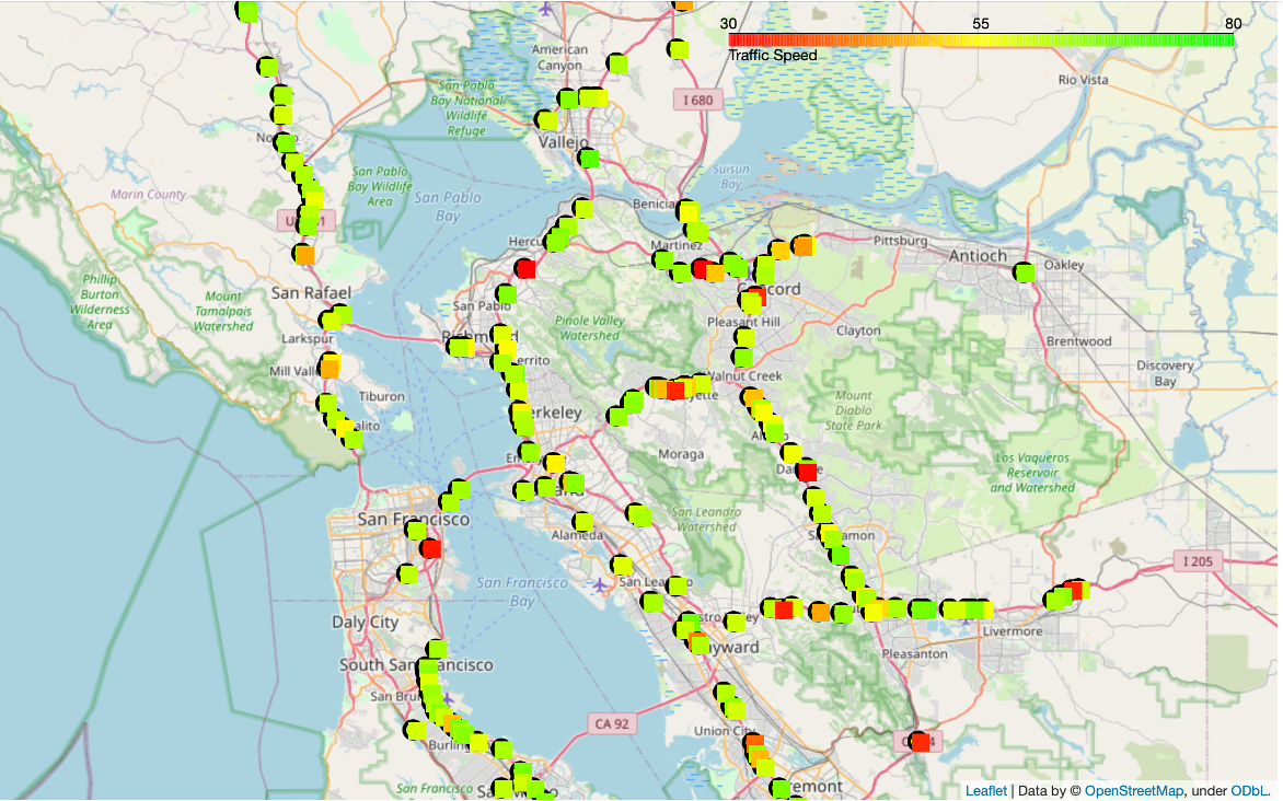
Figure 1: Traffic speed sensing (9:00 pm, 28 January 2021, California, USA)

In this assignment, we are given a set of traffic speed sensor readings (in km/hour) that represent the average traffic speed at 5-minute intervals at different (sensor) locations. The aim is to detect whether there are congestions at each location for the last 5 minutes, and if so, to identify the source of each congestion. You  do not need to be an expert in traffic management or sensor technologies to complete this assignment.

Below is a sample set of input data. The first line contains a positive integer num_locations representing the number of sensor locations in the input data. In the example below, num_locations = 10, meaning that there are 10 sensor locations.

• The last three columns contains IDs of the sensor locations at the “downstream” of the current sensor location, that is, the traffic flows from the current location to these locations. If a column contains a value of -1, it means there are no more downstream sensor locations.

The last line contains two real numbers representing traffic speed thresholds to indicate a congestion, which will be described and used in Stage 3.

The second line of the sample above represents sensor location #104. Its speed limit and latest average traffic speed reading are 80 and 34.31, respectively. Its past average traffic speed readings are: 73.29, 77.35, 66.66, 44.12, 49.65, 60.72, 78.76, 29.45, 15.16, and 35.70.

You may assume that the input is always correctly formatted, and 0 < num_locations < 101. The input is sorted by the sensor location ID in ascending order.

3 Your Task

Write a program that reads the first two lines of the input data and prints out: num_locations, the ID of the first sensor location, the speed limit, the latest average traffic speed, the historical average (HA) traffic speed for the past 10 weeks of the first sensor location, and the IDs of any downstream sensor locations (-1 should not be outputted).

Given a sensor location L with m (m = 10 in our case) past average traffic speed readings s0, s1, . . . , sm−1 (excluding the latest average traffic speed), its historical average traffic speed is calculated as:

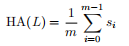
（1）

Here, 53.09 is the historical average traffic speed of the first sensor location as calculated by Equation 1.

You should write functions to process this and the following stages where appropriate.

Hint: To ensure the result accuracy, use double’s for storing the traffic speed readings and calculating the historical average. Use %05.2f for the average speed output formatting. You may also read all input data before printing out for Stage 1.

As this example illustrates, the best way to get data into your program is to save it in a text file (with a “.txt” extension, any text editor can do this), and then execute your program from the command line, feeding the data in via input redirection (using <).

In your program, you will still use the standard input functions such as scanf() to read the data. Inputredirection will direct these functions to read the data from the file, instead of asking you to type it in by hand. This will be more convenient than typing out the test cases manually every time you test your program. Our auto-testing system will feed input data into your submissions in this way as well. To simplify the marking, your program should not print anything except for the data requested to be output (as shown in the output example).

3.3 Stage 3 - Detect Congestions (5 Marks)

Here, location #104 has a speed limit SL = 80. Its latest average traffic speed CL = 34.31 is smaller than α·SL = 0.6×80 = 48.0, while CL is greater than β ·HL = 0.8×53.09 = 42.47. Thus, there is a non-recurring congestion at location #104.

Hint: You should store the HA values calculated in Stage 2 and reuse them for this stage.

3.4 Stage 4 - Detect Sources of the Congestions (4 Marks)

In this stage, we trace back the sources (that is, source locations) of the congestions. When a congestion has been detected at a location L, we examine if any of its downstream locations also has a congestion. If there is a congestion at some downstream location Ld, we further examine the downstream locations of Ld.

The process is performed recursively, until there are no more downstream sensor locations with congestions. The sensor locations that have congestions while their downstream sensor locations do not have congestions are the sources of the congestions, and your program should output these sensor locations. On the same sample input data, the additional output for this stage should be:

• Location #121 also has only one downstream location, #201, which is congested and does not have any further downstream locations. Thus, #201 is another source of the congestion at #104.

Hint: You can use loops instead of recursive functions for this stage, with the help of an array Q to store the sensor locations to be considered. The algorithm to trace the source of a congestion at location L works

5. The loop ends when we reach the last location in Q and there are no more congested locations to beadded to Q.

You may assume that there are no “congestion cycles”, that is, there will not be sensor locations such as

4 Submission and Assessment

This assignment is worth 20% of the final mark. A detailed marking scheme will be provided on LMS. Submitting your code. To submit your code, you will need to: (1) Log in to LMS subject site, (2) Navigate to “Assignment 1” in the “Assignments” page, (3) Click on “Load Assignment 1 in a new window”, and (4) follow the instructions on the Gradescope “Assignment 1” page and click on the “Submit” link to make a submission. You can submit as many times as you want to. Only the last submission made before the deadline will be marked. Submissions made after the deadline will be marked with late penalties as detailed at the end of this document. Do not submit after the deadline unless a late submission is intended. Two hidden tests will be run for marking purposes. Results of these tests will be released after the marking is done.

You can (and should) submit both early and often – to check that your program compiles correctly on our test system, which may have some different characteristics to your own machines.

https://academichonesty.unimelb.edu.au for more information.

Deadline: Programs not submitted by 4:00 pm Monday 2nd October 2023 will lose penalty marks at the rate of 3 marks per day or part day late. Late submissions after 4:00 pm Friday 6th October 2023

will not be accepted. Students seeking extensions for medical or other “outside my control” reasons should email the lecturer at [email protected]. If you attend a GP or other health care professional as a result of illness, be sure to take a Health Professional Report (HRP) form with you (get it from the Special Consideration section of the Student Portal), you will need this form to be filled out if your illness develops into something that later requires a Special Consideration application to be lodged. You should scan the HPR form and send it in connection with any non-Special Consideration assignment extension requests. And remember, C programming is fun!