ECON3020 - ADVANCED MACROECONOMICS
Hello, dear friend, you can consult us at any time if you have any questions, add WeChat: daixieit
ECON3020 - ADVANCED MACROECONOMICS
PROBLEM SET 1
Problem 1: Solow Model with Government Spending [40 marks]
Consider the Solow model without technical progress studied in Lectures 1-2. Suppose that we extended this model by incorporating a government. Specifically, suppose that, in each period  , the government taxes the representative household and uses the proceeds towards “unpro-ductive” government spending
  . The level of public spending is “unproductive”, in the sense that it does not affect the production function that the representative firm operates.
In addition, assume that:
● Government spending is a constant fraction of output:

where
and
is total output in period
● Households save a constant fraction of “private output”, which is defined by
. More precisely, the aggregate level of savings is given by
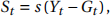
with

● The economy is closed, so that the aggregate resource constraint is
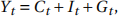
where
is aggregate consumption, and
denotes aggregate investment.
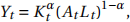
● The representative firm operates the Cobb-Douglas Technology

with

● Capital depreciates at the rate
and the population grows at the rate
> 0.
Answer the following questions, based on this extended version of the Solow model.
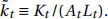
1. Derive an equation that describes the evolution of capital per capita over time.
2. Solve analytically for the level of capital per capita at the steady state. How does capital at the steady state change with
? Provide an intuition.
3. Solve analytically for the levels output per capita, investment per capita, the real wage, and the interest rate in each period, as a function of the stock of capital per capita.
4. For now on, assume that the parameters in the model take the following values:
● The capital share is
= 0.3.
● The population growth rate is
● The depreciation rate is
= 0.1.
● The savings rate is
= 0.2.
● The government spends a fraction of output given by
= 0.15.
Now answer the following questions using Excel:
(a) Solve numerically for the steady state level of capital per capita in the model.
(b) Suppose that the economy is initially in steady state for 10 periods, but afterwards the fraction of government expenditures increases permanently to
Simulate the impact of this shock on the level of capital, output, and investment per capita, as well as on the wage rate and on the interest rate. Explain your findings.
Problem 2: Testing for Dynamic Inefficiency [30 marks]
Consider the overlapping generations model presented in Lecture notes 3-4. Suppose we ex-tend that model by incorporating technical progress. Concretely, assume that the representa-tive firm in the model operates the following technology:
with  where
where  is aggregate output,
  is aggregate capital,
  is labour, and
  repre-sents the level of technology which evolves according to
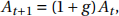
 with g > 0. Assume throughout this exercise that capital depreciates across periods at
 and that the population grows at the rate
  > 0.
> 0.
1. Let
and
denote aggregate consumption at period t of the young and old generation, respectively, so that total consumption at tis
. Show that total consumption in efficiency units of labour satisfies:

where
and
Hint: Begin with the aggregate resource constraint

2. Show that the steady state of this economy is dynamically inefficient if
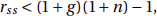
where
is the interest rate at the steady state. Provide a brief intuition for why this
condition is consistent with dynamic inefficiency.
Hint: Dynamic inefficiency holds ifdecreases with
.
3. You will now test whether condition (1) holds in the data for Australia. Follow these steps:
● Download the following series and paste them into an Excel sheet:
– Real GDP per capita data for Australia between 1998-2018. Source: https://data.oecd.org/gdp/gross-domestic-product-gdp.htm.
– Australian population between 1998-2018. Source: https://data.oecd.org/pop/population.htm.
– Long-term interest rates on government bonds for Australia between 1998-2018 (use the annual series) Source: https://data.oecd.org/interest/long-term-interest-rates.htm
● Compute the average annual growth rate of real GDP per capita in Australia between 1998-2018. Use this average to proxy g.
● Compute the average annual growth rate of the Australian population between 1998- 2018. Use this average to proxy n.
● Compute the average annual long term interest rate on Australian government bonds between 1998-2018. Use this average to proxy
Given your estimates above, does condition (1) hold in the data? In other words, is there evidence of dynamic inefficiency in the Australian economy? Provide snapshots of the Excel tables that you constructed.
Problem 3: Pensions in the OLG Model [30 marks]
Consider the overlapping generations model presented in Lecture notes 3-4, and suppose that the government implements a “pay-as-you-go” pension system. Specifically, suppose that young individuals born at  pay a lump-sum contribution
  to the pension system, and the govern-ment transfers such contributions in the form of pensions
  to the old at .
Individuals born at t thus face the following budget constraints:
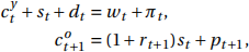
where we apply the same notation used in Lectures 3-4.
The budget of the pension system is balance, so that

Answer the following questions.
1. Assume that individual preferences are represented by the lifetime utility function
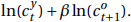
Find an expression for the optimal level of savings as a function of
, and parameters.
2. At a steady state, all per capita variables area constant. In particular,
, where
can be thought of as the size of the pension system. Use this fact to show that optimal savings at the steady state are given by
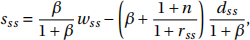
where
is the real wage at the steady state, and
is the interest rate at the steady state.
3. Based on your result from Part 2, how could the government cope with dynamic inef-ficiency by changing the size of the pension system? Explain briefly (you don’t need to provide equations in your explanation).
2021-09-13