QUESTION 1.   Laplace  Transform applied to initial value problems.

Consider the forced vibrational response of a mechanical mass-spring oscillator, such as that used in modelling vehicle suspensions (Case Study 4). The displacement of the mass is given by the following IVP for y(t), t > 0:

d(d) + 2 dt(dy) + 2y = g,     (1A)

subject to

y(0) = y0 ,   y′ (0) = y1 .     (1B)

1.  State the condition for existence and uniqueness of the solution to the above IVP.

2.  Consider the linear algebraic interpretation of the homogeneous IVP (1A-1B) (i.e., the case when g = 0).

(a) Express the IVP as a vector-matrix transformation.

(b) Find a relevant property of the transformation matrix that tells you the type of free vibra- tional response of the system according to:  undamped,  underdamped,  critically damped, overdamped.

(c) Interpret the columns of the transformation matrix, and use these to identify the direction of rotation of the orbits.

(d) Relate the type and stability of the critical point (0,0) to your answer to part (a).

3.  Consider the method of Laplace Transform in solving the IVP (1A-1B).

(a) Find ygeneral , the general solution to the IVP (1A-1B) given

g(t) = sin(at),

y(0) = 1,   y′ (0) = − 1.

You may leave your final answer in terms of a convolution integral:  you are not required to explicitly evaluate the integral.

(b)  Find yh , the homogeneous solution to the IVP (1A-1B) where

g = 0,

y(0) = 1,   y′ (0) = − 1.

(c)  Find yδ , the so-called the impulse response, and the solution to the following IVP

g = δ(t),

y(0) = 0,   y′ (0) = 0.

Interpret g and the boundary conditions.

Note that most textbooks do not bother with δ+ (t) and simply write it as δ(t), as shown for example in your Laplace  Transform  Table.

(d) Prove

ygeneral  = yh + yδ  * sin(at).

4.  Keeping in mind Assignments are helpful to your exam revision, you can check your solution to part 3(b) by solving the system in part 2(a) using Laplace Transform.  This is for practice and will not be marked. A similar question has appeared in a past exam paper.

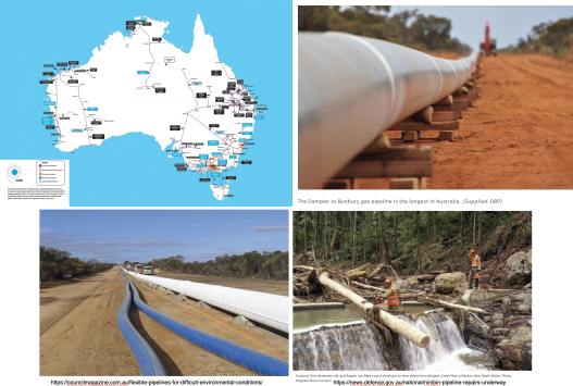
Figure   1:    Case   Study   5A   -   Building   infrastructure   resilience   in   the   face   of   extreme weather  events.    Mathematical  models  assist  in  the  design  of  critical  infrastructure,  like  pipelines  for transport  and  storage  of  gas  and  water  resources,   which  can  withstand  extreme  environmental  condi- tions.  Images from https://councilmagazine.com.au/flexible-pipelines-for-difficult-environmental-conditions/,

https://news.defence.gov.au/national/nimbin-pipeline-repairs-underway, https://www.abc.net.au/news/2021- 03-23/dampier-to-bunbury-gas-pipeline-lifespan-slashed/13239444

QUESTION 2.   Laplace Transform applied to boundary value problems.   The deflection of a buried pipe of length L, located in 0 三 x 三 L, is given by

A d(d)x(4) + Bdx(dy) + Cy = g

where g(x) represents the external force that acts along the pipe from its surrounding medium.

Find y for the following two cases.

1. A downward directed impulse force g is applied at x = , with L = 1, such that

A = 1,   B = C = 0,

and the boundary conditions are

y(0) = y(1) = 0,   y′′ (0) = y′′ (1) = 0.

2.  Near the left boundary x = 0 of a very long pipe, L ≫ 5π, acts a sinusoidal force g, which is governed by the sine function sin(x) turned on along 2π 三 x 三 5π and turned off elsewhere.  The pipe’s deflection due to g near this left boundary simplifies according to:

A = 0,  B = 1,  C = 3,

subject to the boundary condition

y(0) = 2.

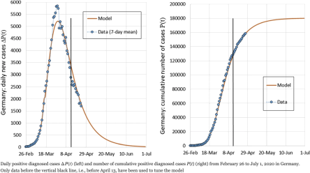
Figure 2:  Case  Study  5B - Epidemic spread.     From Kohler-Rieper et al (2020) A  novel  deterministic forecast model for the  Covid-19  epidemic  based  on  a  single  ordinary  integro-differential  equation.  Eur.  Phys. J. Plus.

QUESTION 3.   Laplace  Transform applied to integrodifferential equations.    The spread of a disease in a local community is monitored.  Data for 0 ≤ t ≤ 2 shows that the rise in the number of infected individuals in a community f(t) is given by the following model

l0 t f(τ)dτ + α + βf = et

subject to

f(0) = ξ .

Find f, given that

α = − 1,   β = 2,   ξ = √2.

Include a plot of f(t) for 0 ≤ t ≤ 2.

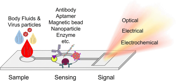
Figure 3: Illustration of microfluidic device used for detecting the genetic material of viruses.  Image sourced from https://link.springer.com/article/10.1007/s42247-021-00169-7

QUESTION 4.  Investigating the representation of discontinuities with Fourier series’.  Microfluidic devices manipulate small volumes of fluid with high precision control and have a diverse array of applications including early diagnosis of SARS-CoV-2 (see for example Tarimetal.  (2021) Microfluidic- based virus detection methods for respiratory diseases.  emergent mater).  The theory of Fourier series is used in the control and interpretation of these experiments (see for example equation 10 of https:  //doi.org/10.1039/B718376C)

(a)  Consider the following function and its periodic extension:

f(x) = |sinx| ,        where         < x ≤        and       F(x) = f(x + nπ),        where       n ∈ Z Find the Fourier series representation of F(x).  Note that L =  .

(b)  Does the Fourier series you found in (a) converge uniformly? If so, prove this using the Weierstrass test for uniform convergence.   If  not,  discuss whether  it converges pointwise anywhere in its domain.

(c)  Use your result in (a) to evaluate the following two series

        and         4n1 .

(d) Attempt to differentiate your Fourier series in (a) term by term. Does the resulting series converge uniformly?  If so, prove this using the Weierstrass test for uniform convergence.  If not, discuss whether it converges pointwise anywhere in its domain.

(e)  Carefully differentiate the function F(x), as defined in (a), and then find the Fourier series of the resulting function, i.e., find the Fourier series of F′ (x).

(f) Write 1-2 sentences comparing your series’ from (d) and (e), discussing how well the term by term differentiation has worked.

(g) Attempt to differentiate your Fourier series in (d) term by term. Does the resulting series converge uniformly?  If so, prove this using the Weierstrass test for uniform convergence.  If not, discuss whether it converges pointwise anywhere in its domain.

(h)  Carefully differentiate your answer from  (e),  and then find the Fourier series of the resulting function, i.e., find the Fourier series of F′′ (x). You may reuse working from previous questions.

(i) Write 1-2 sentences comparing your series’ from (g) and (h), discussing how well the term by term differentiation has worked.