The objective of this assignment is to provide you an opportunity to implement some of the  existing  image  reconstruction  algorithms  using  Matlab.  You  are  required  to implement your own back projection algorithm and filtered back projection algorithm    to reconstruct the image using based on the given sinogram data, g( ,θ) .

About the Sinogram

You are given a set of data that corresponds to the sinogram of an image, i.e. g( ,θ ) . Type “load(128_ 18.mat) and “size(sino)” in Matlab environment, it would show “185 18”, which means that the size of the array is 185 rows x 18 columns. Physically, this means  that  the  sinogram is  formed  based  on   185 parallel   beams (-92=   =   93) projecting onto the object. The projections are taken from 18 snap shots ranged from 10 to 180 degree with the step size of 10 degrees.

About the Reconstructed Image

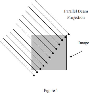
1. The reconstructed image will be in an array size of 128 x 128 while the width of the projection is 185. In parallel-beam projection, each projection has to cover the whole area-of-interest, including in the diagonal position (e.g. 45。) shown in the Figure  1. Thus the parameter     in the Sinogram has to be at least equal to the diagonal of the image.

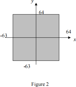
2. The reconstructed image would be in the rectangular coordinates with x and y ranges from -63 to 64 (Figure 2).

Based on the given Sinogram, together with the teaching materials, complete the following tasks:

Part A. Back-projection

A1.  Write  down  the  expression  of  the  back-projection  and  explain  the  physical meaning of each term in the equation.

A2. Compute and plot the back projection of the image at  θ = 30° .

A3. Compute and plot the back projection summation image. Multiply the resultant image by the factor of π/(2 × PN), where PN is the number of back projections (PN= 18).

B. Filtered Back Projection (FBP)

B1.  Draw  a  flow  chart  to  illustrate  the  steps  to  compute  the  FBP  based  on  the sinogram data. List out the relevant expressions, and explain how these equations related to each other.

B2. Similar to A3, implement the FBP algorithm and plot the reconstructed images. Multiply the resultant image by the factor of π/(2 × PN).

C. Quantifying the Image Reconstruction Outcomes

To quantify the quality of the reconstructed images, mean square error (MSE) between the reconstructed images and the original image can be computed:

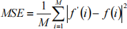
where  f ' (i) is the reconstructed image, and   f (i) is the original image. The index i corresponds  to  the  pixel  number  of  the  image  and   M   corresponds  to  the  total number of pixels.

C1. Load ‘original_image_ 128.mat ’. Compute the MSE for the reconstructions that you have obtained in A3 and B2.

C2. As a benchmark, use the command ‘iradon ’ to reconstruct the image. If your reconstruction image, it will be in the size of 130 x 130. Remove the first row, first column, last row and last column such that the reconstructed image is now in the size of 128 x 128. Compute the corresponding MSE using the Matlab command ‘immse ’. 

C3. Instead of using the data set “128_ 18.mat”, use the data set “128_60.mat” and reconstruct your images using back projection (A3) and filtered back projection (B2). In summary, you should have 6 reconstruction results with 6 MSE values (Table 1)

Table 1. MSE of image reconstruction results using 18 and 60 projections

C4. Compare and comment on the results.

D. Algebraic Reconstruction Technique

Algebraic Reconstruction Technique (ART) formulates the reconstruction problem as solving a system of linear equations, given by

[w][f] = [p],                                                 (1)

where  [w]  is the weighting matrix describing the contribution of every cell for all the different rays  in  each projection,  [f]  represents  the  unknown  pixel  values  of the images and  [p]  is the obtained projection data. The image reconstruction problem is equivalent to the solution of linear system in (1).

One way to solve (1) is to use the Kacamarz’s method which uses an iterative procedure  to  determine  the  unknown   [f] .  The  implementation  of  ART  can  be expressed as

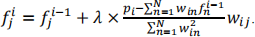                              (2)

The  subscript  j  corresponds  to  the  pixel  number  of  the  image  that  we  want  to reconstruct (fi ) while i  corresponds to the number of the projection data (pi ). In each update (from fi−1  to fi ), the correction value is calculated based on the difference between measured projection data and the calculated projection from line integral of pixel value f. λ  is known as the relaxation factor, which is used to control the impact of the correction factor.

You are given a number of m files and a Matlab GUI that allows you to perform image reconstruction using ART.

D1. Execute the m file “ART_GUI.m” (not ART_GUI.fig). You will then see a GUI pops out. Click on the “Import Sinogram” button and select the ‘128_ 18.mat ’ file and load it into the program.

D2. To start using the ART GUI, do the following settings:

Note: The SNR is set to “inf” such that there is no random noise introduced. Do not choose “50*50” and the “line-based model” . You need to install the “Communications Toolbox” for your MATLAB to be able to run some of the functions. You may also      need a relatively large memory (e.g. > 10Gb) to run the program properly. Use the UQ Digital Workspace if needed (see Ed Discussion for instruction).

Once you have got the setting ready, press “reconstruct” to perform the reconstruction. Press “Save Data” and save the image as “128_ 18_N=5.mat” .

Compute the MSE value and put it in Table 2.

D3.  To  numerically  evaluate  the  reconstruction  process,  repeat  D2  with  different iteration numbers (N). Set N from  1 to  10 and compute the corresponding the MSE. For convenience, you may wish to save the file as 128_ 18_N=iteration_number.mat (e.g. 128_ 18_N=3.mat) such that you can reload the results when needed.

D4. Repeat D2  and  D3 with  “128_60.mat” .  In  summary,  you  should  have  all  the results listed in Table 2. Graphically, plot the results in Table 2 (MSE vs Iterations Number, one for PN=18 and one for PN=60)

Table 2. MSE vs iteration number (N) of the ART image reconstruction results using 18 and 60 projections

D5. Comment on the findings that you have got D4. Compare the results in D4 and your earlier findings in C3 and C4. How does ART perform as compare to Filtered Back projection and inverse radon transform? Comment your answer in terms of (i) the image reconstruction performance of ART as a function of iteration number; (ii) comparison between the optimal ART results with Filtered Back Projection when the projection number is increased from 18 to 60.

E. Further readings

E1. The relaxation factor, λ,controls the impact of the correction factor and thus the  convergence of ART. Have a look at the literature to find out relevant studies on how the relaxation factor would impact the convergence of ART. In your answers, you are required to provide the relevant reference(s) that supports your answer.

E2. To verify your findings in E1, use different values of relaxation factor, together with the program, generate at least two  sets  of data  (MSE vs  iteration number) to support  your  findings.  Does  your  finding  agree  with  what  was  reported   in  the literature?

D4       Summary  of the  MSE  of D2 and D3 and present as Table 2,

Matlab code for computing the MSE

D5       Comments for (i) and (ii)

E1       Explanation and reference(s)

E2       Simulation Results and explanation

Table 3. Details for Report Submission

PS: Matlab Code: Program listing in the report, m file and related data files (.mat) that generates the results are required.