Hello, dear friend, you can consult us at any time if you have any questions, add WeChat: daixieit

MATH4090: Computation in Financial Mathematics

Assignment 1

Semester II 2023

Due 5:00pm 21 August 2023                        Weight 20%

Total marks                                                    40 marks

Submission instructions:

❼ Submit onto Blackboard softcopy (i.e. scanned copy) of (i) your assignment solutions, as well as (ii) Matlab code, if any, by 5:00pm 21 August 2023. Hardcopies are not required.

❼ You also need to upload all Matlab files onto Blackboard.

General coding instructions:

❼ You are allowed to reuse any code developed in tutorials.

❼ An assignment question may have specific programming instructions which you are required to follow. Failure to do so will result in a loss of 50% of the questions’s total marks.

❼ For programming questions that require you to submit tables of results, you are not required to write Matlab code to produce the tables. Handwritten tables of results are acceptable.

Notation: “Lx.y” refers to [Lecture x, Slide y]

Assignment questions

For Questions 1 and 2, please refer to the supplementary notes on the no-arbitrage binomial tree method located in the ’Lecture set 1’ folder. These notes provide a more detailed explanation of the binomial tree method that was discussed during the lectures and tutorials.

1. (2 marks) Recall that we let N be the number of time periods of the tree, where N is a positive integer. In addition, Sjn, 0 ≤ n ≤ N, −n ≤ j ≤ n, is the price of the underlying asset at node (n, j) of the tree.

Mathematically prove the following:

Programming instructions for Question 1: This is not a programming question.

2. (10 marks) Consider a T-maturity European-style financial product whose payoff is given by

where K > 0. Here, ST denotes the price of the underlying asset at maturity.

To price this financial product, we use the no-arbitrage binomial tree method discussed in class. We let N be the number of time periods of the tree, where N is a positive integer.

Recall that Sjn, 0 ≤ n ≤ N, −n ≤ j ≤ n, is the price of the underlying asset at node (n, j) of the tree. We denote by Pjn, 0 ≤ n ≤ N − 1, −n ≤ j ≤ n, the numerical price of the aforementioned financial product at node (n, j) obtained by the no-arbitrage binomial method. In particular, P0 0 is the no-arbitrage price of the financial product at (S0, t0).

(a) (5 marks) Use induction to prove that

Hint: Use the result in (1).

Programming instructions for Part (a): This is not a programming question.

(b) (5 marks) You are asked to numerically verify (3) at node (n, j) = (0.0).

Outline a binomial method to estimate P0 0 . Implement your proposed method in Matlab.

Programming instructions for Part (b): This is a programming question with the following instructions.

❼ Your code must consist of (i) a function named bi tree.m which computes P0 0 or a fixed N, and (ii) a Matlab script file named test bi tree.m that uses this function.

❼ You should compute P0 0 by conducting a backward induction in the tree, starting from the payoff defined by (2), and subsequently compare this with (3).

❼ The parameters for the options are: T = 1, σ = 0.3, S(0) = 100, r = 0.02, K = 100.

❼ In the numerical experiments, for the number of time periods N in the binomial tree, use N = Nk = 50 × 2 k , k = 0, 1, . . . 8. We further denote by P0 0,k ≡ P0 0 (∆t)k, k = 0, 1, . . . 8, numerical approximations to the true price P(S0 0 , t0), noting S0 0 = S0 and t0 = 0, using the tree method with the timestep size (∆t)k = T /Nk.

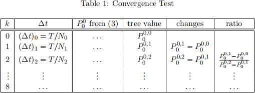
❼ Fill in Table 1 above. Submit your code, together with the output, observations and comments.

3. (8 marks) For this question, you are asked to implement the (no-arbitrage) binomial tree pricing algorithm for American put options discussed in L1 and Tutorial 3.

Programming instructions for Question 3: This is a programming question with the following instructions.

❼ Similar to Question 2, you will need to submit two Matlab files, namely a function named bi tree amer.m which computes an approximation to the true option price for a fixed N, and (ii) a Matlab script file named test bi tree amer.m that uses this function.

❼ Take the following parameters: T = 0.25, σ = 0.8, S(0) = 100, r = 0.1, K = {97, 100}.

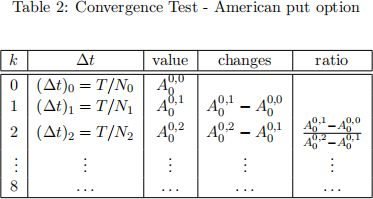
❼ For the number of time periods N in the binomial tree, use N = Nk = 100 × 2 k , k = 0, 1, . . . 8. We denote by A00,k ≡ A00 (∆t)k, k = 0, 1, . . . 8, numerical approximations to the (unknown) true price of the American put option at S0 0 = S(0) and time t0 = 0 using the tree method with the timestep size (∆t)k = T /Nk. We denote the true price at node (n, j) by A(Sjn, tn).

❼ Fill in Table 2, one for each value of the strike price K. Submit your code, together with the output, observations and comments.

In general, a closed-form solution for the price of an American put option does not exist. For the above set of parameters, when K = 100, a very accurate price, which is obtained by another computational method, is 14.6788877. You can use this value as benchmark.

What do you observe from the “ratio” column in these two tables?

4. (10 marks) In this question, we consider two American options.

❼ The first option is a TD-maturity and KD-strike American put option written on a stock S, where TD > 0 and KD > 0 are fixed. We will refer to this option as the daughter (D) option.

❼ The second option is a TM-maturity and KM-strike American put written on the daughter option, where 0 < TM < TD and KM > 0. We will refer to this option as the mother (M) option.

Specifically, on the interval [0, TD], the daughter option gives its holder the exercise privilege at strike KD with the stock S being its underlying, whereas, on the interval [0, TM], the mother option gives its holder the early exercise privilege at strike KM with the daughter option being its underlying. Note that the holder of the mother option is not necessarily the same as the holder of the daughter option.

a. (5 marks) Denote by Mjn and Djn the price at node (Sj , tn) for the mother and daughter options, respectively. Describe a binomial tree method to price the mother option.

Programming requirements: This part is a non-programming question.

b. (5 marks) Code in Matlab the binomial tree method you proposed in Part (a). For numerical experiments, take the following parameters: TD = 1.0, KD = 100, TM = 0.5, KM = 4, σ = 0.1, S(0) = 100, r = 0.02, For the number of time periods N in the binomial tree, use N = Nk = 100 × 2 k , k = 0, 1, . . . 8. We further denote by M0 0,k ≡ M0 0 (∆t)k,

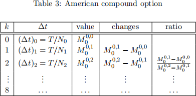
k = 0, 1, . . . 8, the numerical approximation to the (unknown) true price M(S0 0 , t0), noting S0 0 = S0 and t0 = 0, using the tree method with the timestep size (∆t)k = T /Nk.

Programming requirements for Part (b): This part is a programming question with the following instructions.

❼ You must have a function named in bi tree compound.m which computes an approximation to the (unknown) true mother option price for a fixed N.

❼ You also need to write a Matlab script file that uses this function. Name this script file test bi tree compound.m.

Fill in Table 3. Submit Matlab files, together with your output, observations and comments.

5. (10 marks) Let C(S0, K, T) be the time-0 price of a European call option with maturity T and strike K written on the underlying asset following Merton jump-diffusion dynamics with S0 being the time-0 asset price3 . This price is given by the analytical expression:

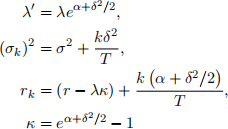
Here,

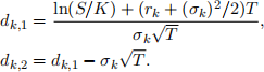
and CBS (S0, K, rk, σk, T) denotes the Black-Scholes formula for a European call option. It is given by

C BS (S0, K, rk, σk, T) = S0N (dk,1) − Ke−rkT N (dk,2),

where N(x) is the cumulative distribution function (CDF) of the standard normal distribution, defined by

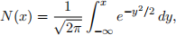
and

In the above expressions, r > 0 and σ > 0 are the risk-free rate and the instantaneous volatility, respectively; λ ≥ 0 is a constant finite jump intensity (jumps arrive according to a Poisson process with rate λ); α and δ 2 respectively are the mean and the variance of a normal random variable representing the jump multiplier. (If a jump occurs at time t, then the underlying asset price after the jump is ξSt , where ξ ∼ Normal(α, δ2 )). Each term CBS (S0, K, rk, σk, T) in (4) is the value of the option conditional on there being exactly k jumps during its life.

Your task is to implement in Matlab the pricing formula in (4) for a European call option written on Merton jump-diffusion dynamics.

Programming instructions for Question 5: This is a programming question with the following instructions.

❼ Your code must consist of (i) a function named Merton call.m which computes C(S0, K, T), and (ii) a Matlab script file named test Merton call.m that uses this function.

❼ The function Merton call.m takes the following input arguments (S0, K, r, σ, T, λ, α, δ).

❼ In the function Merton call.m, you need to implement the infinite series using a loop over k. The loop should stop if the k-th term of the series is less than 10−8 . (Try to convince yourselves that the loop should stop after a finite number of iterations.)

❼ The parameter values for testing are: S0 = 100, K = 100, T = .25, r = 0.03, σ = .2, λ = 1, α = 0.5, δ = 0.1.