Overall Description

In this assignment, you will be asked to implement code and perform experimentsI(˙)n general, this

assignment has two parts, each of them graded as follows:

1.  Stream Learning (18 marks)

2.  Continual Learning (7 marks)

IMPORTANT. AI Tools (like ChatGPT, CoPilot, Bard, and others) should not be used to answer the questions or code the assignment. If you want to use a tool to improve your writing of the report, Grammarly is a better option than the other AI tools.

.  Use MOA or River for the Stream learning part and Avalanche for the Continual Learning part.

. Your code should be compatible with either MOA or river for the Stream Learning part. If you want to use some other library (like scikit-multiflow) or code everything from scratch1  talk to the lecturer first.

.  There is a template code that you must use for the Continual Learning part.

.  Throughout this assignment, there are (Optional) questions, experiments and variations. These do not grant you extra marks.  These are challenges that may go beyond what was taught in the course or require more coding and analysis efforts. You are encouraged to try them, but you are not required to so.

. Your submission must contain the following files.  Do not forget to submit anything, double check before moving on!  Also make sure you are submitting to the right paper!

1.  (Stream Learning) a file containing the classifier implementation (a single .java or .py);

2.  (Continual Learning) a Jupyter notebook containing the implementations (follow the tem- plate);

3.  (Stream Learning and Continual Learning) a single pdf report with the experiments and answers;

4.  a README file with details about how to run your code and reproduce the experiments. Notice that a jupyter notebook doesn’t replace the PDF report, if you decide to use Python for the Stream Learning part, you are still required to submit the PDF report. Similarly, for the Continual Learning part, make sure to add the plots and other results to the PDF report.

1    Stream Learning

You must code a new ensemble classifier, but you are encouraged to look at the existing ensemble classifiers to observe how base learners are usually stored, hyperparameters conventions, and other common code. Notice that your ensemble classifier must be implemented in either MOA or river in a way that it can be executed as a stand-alone classifier.  The ensemble must contain the implementations to satisfy the requirements described in the following subsections.

1.1    Coding the ensemble  [10 Marks]

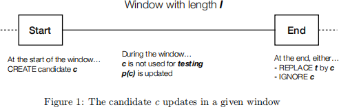
The ensemble will have a fixed number of learners S.  Updates to the ensemble (i.e.  additions and removals) will occur every l instances, such that these can be identified as windows of length l instances. At the start of each window, a new base model should be added as a candidate c to join the ensemble. At the end of each window, the ensemble will either:  REPLACE another learner e currently in the ensemble by c; or IGNORE c and discard it. This process is depicted on Figure 1.

The base learner for the ensemble will be the Hoeffding Tree algorithm.  (Optional):   You  are encouraged to  think about how your ensemble  could be implemented using  any base learner,  but that is not mandatory.  The majority of the ensemble algorithms available in MOA/river do not enforce the use of a specific base learner.  However, it would be not easy to accomplish that in this assignment as the diversity induction strategy assumes that we are using a Hoeffding Tree.

The training and testing methods depend on how diversity is induced (see 1.1.4) and the voting method  (see 1.1.2).   Notice that even though the ensemble is updated in windows of length l, the Hoeffding tree models are continuously updated, i.e.  they should not be reset after processing every window and they should be updated during the window as well.

Feel free to name your algorithm, but if you cannot find a good name, just call it Streamzilla  (we will refer to it using this name).

1.1.1    Predictive performance p(e)

The estimated predictive performance p(e) of each member e of the ensemble E must be stored and continuously updated.  Concretely, immediately before using an instance xt  for training an ensemble member e, xt  should be used for assessing whether e would correctly predict it,i.e.  he (xt ) = yt.  Notice that if the instance xt  is first used for training e, then the estimated predictive performance would be misleading.  By default, p(e) corresponds to the accuracy of e, i.e.  number of correct predictions divided by total number of predictions made by e.   (Optional):   Encapsulate p(e) such that other metrics, such as Kappa T, could be used.

1.1.2    Prediction - Weighted votes

The ensemble prediction should be determined by a weighted majority vote strategy.  The weights of each member e are determined according to the predictive performance p(e).

During prediction, the algorithm should sum the weighted votes assigned to each class label to decide the ensemble prediction.  For example, given an ensemble with four models, such that p(g) = 0.90, p(m) = 0.85, p(n) = 0.81, and p(q) = 0.92, where the predictions for a given x were hg (x) = 0, hm (x) = 0, hn (x) = 0, and hq (x) = 1.  The weighted votes for class 0 w(0) = 0.90 + 0.85 + 0.81 = 2.56 and for class 1 w(1) = 0.92, as a consequence, the ensemble prediction is class 0.

1.1.3    Dynamic updates

After processing l instances, the algorithm should be updated by replacing the worst e*   (min p(e)) by the new model c.  If p(c) ≤ p(e* ), i.e.  the predictive performance of c is worst than the minimum predictive performance observed in the ensemble p(e* ), then c should be discarded (i.e. IGNORED).

1.1.4    Training - Inducing diversity

There are multiple ways of inducing diversity into an ensemble model  [1].   One can vary in which instances or features the models will be trained,  modify the outputs of the training instances,  or even combine several strategies. In this assignment, you are asked to implement a strategy that vary the hyperparameters of the base Hoeffding Trees.  Concretely, implement a method that create new candidate trees c with random values for the following hyperparameters.

.  Grace period gp.  The number of instances a leaf should observe between split attempts.  Range of values (10; 200).  Step = 10.

.  Split Confidence sc.  The allowable error in split decision. Range of values (0.0; 1.0).  Step = 0.05.

.  Tie Threshold t.  Threshold below which a split will be forced to break ties.  Range of values (0.0; 1.0). Step = 0.05.

For example, a given c may be initialized with gp = 110, sc = 0.05 and t = 0.55.  There is not much difference between a tree trained using sc = 0.046 and sc = 0.05, thus we define a step of 0.05 for sc and t, and a step of 10 for gp.

1.2    Evaluation and Analysis  [8 marks]

The results should be presented using a table format, followed by a short analysis about them guided by the questions associated with each experiment.  More details are presented in the subsections for each experiment.

Evaluation framework. For all experiments, use a test-then-train evaluation approach and report the final result obtained, i.e.  the result obtained after testing using all instances.  When required to plot, you should use prequential evaluation (use a window of 1,000 instances) and plot results every 1,000 instances (sample frequency parameter in MOA).

Evaluation Metrics. Unless specified otherwise, for all experiments, report accuracy and pro- cessing time2 .

Datasets.    electricity,  covertype,  SEA abrupt  (drift  at  50000),  SEA gradual  (drift  at  50000, width=10000), and RTG 2abrupt (drift at 30000 and 60000) .  Refer to attached materials to obtain the “.arff” and “.csv” versions.

1.2.1    Experiment 1:  Streamzilla variations and sanity check  [4 marks]

In the first part of the evaluation, you are asked to perform experiments using Streamzilla and a single Hoeffding Tree.  This experiment will produce 3 Tables of results  (algorithms  (columns) vs datasets (rows)),where S = K represents the number of learners, seed is the initializer to the random object3 , and l is the length of the window.   Important:  you  don’t need to report the time taken for this experiment as it would require yet another run.

.  First table (l = 1000 for all Streamzilla variations): HoeffdingTree, Streamzilla(S = 5),Streamzilla(S = 10), Streamzilla(S = 20), and Streamzilla(S = 30);

.  Second table  (S  =  20  and  l  =  1000  for all):  Streamzilla(seed  =  1),  Streamzilla(seed  =  2), Streamzilla(seed = 3), Streamzilla(seed = 4), Streamzilla(seed = 5)

.  Third table (S = 20 for all):  Streamzilla(l = 500), Streamzilla(l = 1000), Streamzilla(l = 2000), Streamzilla(l = 5000), Streamzilla(l = 10000)

Guiding Questions experiment 1:

1.  How does  Streamzilla compares against a single Hoeffding Tree?   Also,  does  Streamzilla  im- prove results  if more base models  are  available?   Present  a  table  with  results  varying  from S = {5, 10, 20, 30}, where S is the total number of learners.

2.  Can Streamzilla recover from concept drifts?  Present a plot depicting the accuracy over time to support your claim. There should be a plot for each dataset comparing whichever version of Streamzilla that produced the best results on the first table against the single Hoeffding Tree.

3. What is the impact of the l hyperparameter? Discuss the results varying the l hyperparameter. You can define l based on your intuition, but at lest 3 variations should be present representing a small l, a reasonably sized l and a large l.

4.  (Optional) Which combination of l and S presents the best results for each dataset (on average). This will require another separate table where variations of l and S are combined together.

Important:  To generate the results to be plotted you should use the Prequential evaluation.  In MOA, EvaluatePrequential with its default Evaluator should be sufficient. The code from the following repository can be used for the plots, but notice that any other tool or language can be used.

https://github.com/hmgomes/data-stream-visualization

1.2.2    Experiment 2:  Streamzilla vs.  others [4 marks]

Compare the best result of Streamzilla, obtained in the previous experiment, against Adaptive Random Forest (ARF)  [2] and Dynamic Weighted Majority (DWM)  [4] (Update:  use  Online Bagging[6] for River) for each dataset.  Use S = 20 (number of base learners) for all the ensembles, subspace m = 60% for ARF and default hyperparemeters for DWM. This will produce two tables with results:

.  First table: The accuracy for each ensemble and dataset.

.  Second table: The processing time for each ensemble and dataset.

Guiding questions for experiment 2:

1.  How does Streamzilla performs in terms of predictive performance against the others?

2. In terms of processing time, is Streamzilla more efficient than the other methods?  If not, what is the most efficient one?

3.  Create another table varying the number of base learners in the other datasets as well.  Then discuss which ensemble method scales better in terms of accuracy, i.e.  produces better results as we increase the number of base learners for the given datasets.  Experiment with at least 3 configurations for each ensemble (e.g.  S  ∈ {10, 20, 30}), notice that some of them you might already have the results from the previous experiments.

4.  (Optional) What design choice made affects the computational resources the most for Streamzilla? For example, one design choice is how the algorithm update learners, another one is how diversity   is induced, and there are many others. Notice that the value of l or S is not a design choice, it   is an hyperparameter configuration.

5.  (Optional) What design choice of ARF impacts its computational performance the most?

2    Continual Learning  [7 marks]

In this part of the assignment, you will be asked to use the Avalanche library to perform some ex- periments using the Fashion-MNIST dataset. We are assuming a class-incremental setting in this exercise.   You  must  use  the template Jupyter notebook available on the assignments webpage to prepare your implementation.  Finally, remember to create a separate MLP model for each continual learning strategy (i.e. the strategies shouldn’t share the same MLP model).

2.1    Experiment 1:  Analysing the baseline strategies [3 marks]

Execute the train loop using the baseline strategies Naive and Cumulative to answer the following questions.

1.  Plot the Confusion matrix for each strategy and the accuracy on all tasks after training on the final task.

(a) What can be concluded from observing the Confusion matrix and accuracy on all tasks after training on each task for the Naive strategy?

(b) Which strategy yields a better overall accuracy 4  and why it happens?  Comment on the validity of using such strategy in a practical continual learning setting where memory and processing time are scarce.

2. Is it possible to significantly improve the accuracy of the strategy that did not perform very well in the previous experiment by changing or tuning the learning model? If your answer is yes, add an experiment that shows that the accuracy can be significantly improved.  If your answer is no, then justify it based on the characteristics of the strategy.

2.2    Experiment 2:  Analysing other CL strategies [4 marks]

Experiment with the strategies Elastic Weight Consolidation (EWC) [3] and Gradient Episodic Memory (GEM) [5] to answer the following questions.

1.  Report only the  overall  accuracy  (after  training  on  the  last  task)  for  at  least  3  different values for the hyperparameters patterns per exp (GEM) and ewc lambda  (EWC).  Compare the results  (overall accuracy) against the Naive and the Cumulative strategies and discuss them.  Hint:  Do not report the Confusion matrices and accuracy for all tasks after training on each of them for this experiment.

2.  Select the best strategy between GEM and EWC and configuration from the previous experiment (according to the overall accuracy), and attempt to increase its overall accuracy even further by improving the learning model.  Concretely, you should attempt at least one different architecture for the SimpleMLP (i.e.  different number of hidden layers, different value for dropout, ...)  and try to increase the train   epochs.  Hint:  Watch out for too complex models and too large values of train   epochs as these can take too long to train.

(a)  A more complex MLP model guarantees improvements in the overall accuracy?  Discuss your answer based on your experiment.

(b)  Increasing the train  epochs guarantees improvements in the overall accuracy? Discuss your answer based on your experiment.

3.  (Optional) Try to improve the accuracy results even further by using another continual learning strategy or by improving the learning model (e.g. by adding more layers, changing it to a more complex model, using another optimiser, ...).

4.  (Optional) Report the time and memory needed to train GEM and EWC and discuss which method is more efficient.

4 i.e.  Top1 Acc Stream/eval phase/test stream/

3    Submission

3.1    Datasets

The relevant data files can be found as a .zip file on the course wiki.  For the CL part, the dataset will be automatically downloaded.

3.2    Submission Method

The code, report and README should be submitted through the web submission system for AIML431 by the due time.

Notice that you can submit a .zip file to preserve the subdirectory structure you might have created to organise your submission.

Please  check  that  your  programs  can  be  run  on  the  ECS  machines  easily  according  to  your README. If we can’t run your code, you may  lose  marks!   We have a limited amount of time (¡ 5 minutes) to get your code running. It should be straightforward to run your code for the Stream Learning part using either MOA or river, and for the CL part you shouldn’t deviate from the Avalanche Jupyter notebook template.

3.3    Late Submissions

The assignment must be submitted on time unless you have made a prior arrangement with the lecturer or have a valid medical excuse.  We use the ECS extension system for all extension requests.  Please make a request there if you think you have a valid reason.

3.4    Plagiarism

Plagiarism in programming (copying someone else’s code) is just as serious as written plagiarism, and is treated accordingly. Make sure you explicitly write down where you got code from (and how much of it) if you use any other resources asides from the course material.   Using  excessive  amounts of others’ code may result in the loss of marks, but plagiarism should result in zero marks and other consequences.