1 Setup

Consider the following problem: an agent in a gridworld has to move from its current cell to the given cell of a non-moving target, where the gridworld is not fully known.  They are discretizations of terrain into square cells that are either blocked or unblocked.

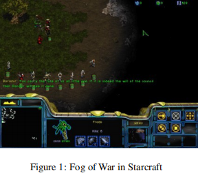
Similar search challenges arise frequently in real-time computer games, such as Starcraft shown in Figure 1, and robotics. To control characters in such games, the player can click on known or unknown terrain, and the game characters then move autonomously to the location that the player clicked on.  The characters observe the terrain within their limited field of view and then remember it for future use but do not know the terrain initially (due to “fog of war”).  The same situation arises in robotics, where a mobile platform equipped with sensors builds a map of the world as it traverses an unknown environment.

Assume that the initial cell of the agent is unblocked.  The agent can move from its current cell in the four main compass directions (east,south, west and north) to any adjacent cell, as long as that cell is unblocked and still part of the gridworld. All moves take one time step for the agent and thus have cost one. The agent always knows which (unblocked) cell it is in and which (unblocked) cell the target is in. The agent knows that blocked cells remain blocked and unblocked cells remain unblocked but does not know initially which cells are blocked.  However, it can always observe the blockage status of its four adjacent cells, which corresponds to its field of view, and remember this information for future use. The objective of the agent is to reach the target as effectively as possible.

A common-sense and tractable movement strategy for the agent is the following: The agent assumes that cells are unblocked unless it has already observed them to be blocked and uses search with the “freespace assumption”. In other words, it moves along a path that satisfies the following three properties:

1.  It is a path from the current cell of the agent to the target.

2.  It is a path that the agent does not know to be blocked and thus assumes to be unblocked,i.e., a presumed unblocked path.

3.  It is a shortest such path.

Whenever the agent observes additional blocked cells while it follows its current path, it remembers this information for future use.  If such cells block its current path, then its current path might no longer be a “shortest presumed-unblocked path” from the current cell of the agent to the target.  Then, the agent stops moving along its current path, searches for another “shortest presumed-unblocked path” from its current cell to the target, taking into account the blocked cells that it knows about, and then moves along this path. The cycle stops when the agent:

• either reaches the target or

•  determines that it cannot reach the target because there is no presumed-unblocked path from its current cell to the target and it is thus separated from the target by blocked cells.

In the former case, the agent reports that it reached the target.  In the latter case, it reports that it cannot reach the target. This movement strategy has two desirable properties:

1.  The agent is guaranteed to reach the target if it is not separated from it by blocked cells.

2.  The trajectory is provably short (but not necessarily optimal).

3.  The trajectory is believable since the movement of the agent is directed toward the target and takes the blockage status of all observed cells into account but not the blockage status of any unobserved cell.

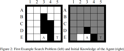
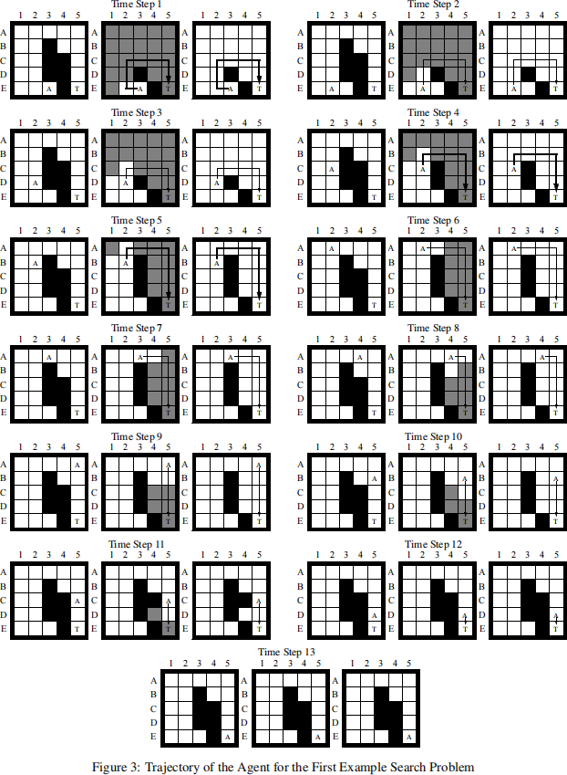
As an example, consider the gridworld of size 5 × 5 shown in Figure 2 (left). Black cells are blocked, and white cells are  unblocked. The initial cell of the agent is marked A, and the target is marked T. The initial knowledge of the agent about  blocked cells is shown in Figure 2 (right).  The agent knows black cells to be blocked and white cells to be unblocked.  It does not know whether grey cells are blocked or unblocked.  The trajectory of the agent is shown in Figure 3.  The left  figures show the actual gridworld. The center figures show the knowledge of the agent about blocked cells. The right figures  again show the knowledge of the agent about blocked cells, except that all cells for which it does not know whether they  are blocked or unblocked are now shown in white since the agent assumes that they are unblocked.  The arrows show the  “shortest presumed-unblocked paths” that the agent attempts to follow. The agent needs to find another “shortest presumed-  unblocked path” from its current cell to the target whenever it observes its current path to be blocked. The agent finds such  a path by finding a shortest path from its current cell to the target in the right figure. The resulting paths are shown in bold  directly after they were computed. For example, at time step 1, the agent searches for a “shortest presumed-unblocked path” and then moves along it for three moves (first search).  At time step 4, the agent searches for another “shortest presumed-  unblocked path” since it observed its current path to be blocked and then moves along it for one move (second search). At  time step 5, the agent searches for another “shortest presumed-unblocked path” (third search), and so on. When the agent  reaches the target it has observed the blockage status of every cell although this is not the case in general.

2 Modeling and Solving the Problem

The state space of the search problem arising is simple:  The  states correspond to the cells, and the actions allow the agent to move from cell to cell.  Initially, all action costs are one.  When the agent observes a blocked cell for the first time, it increases the action costs of all actions that enter or leave the corresponding state from one to infinity or, alterna- tively, removes the actions. A shortest path in this state space then is a “shortest presumed-unblocked path” in the gridworld.

Thus, the agent needs to search in state spaces in which action costs can increase or, alternatively, actions can be removed. The agent searches for a shortest path in the state space whenever the length of its current path increases (to infinity). Thus, the agent (of the typically many agents in real-time computer games) has to search repeatedly until it reaches the target. It is therefore important for the searches to be as fast as possible to ensure that the agent responds quickly and moves smoothly

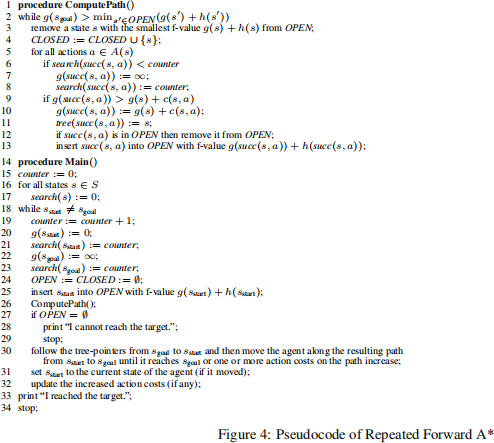
The pseudocode of Repeated Forward A* is shown in Figure 4. It performs the A* searches in ComputePath(). A* is described in your textbook and therefore only briefly discussed in the following, using the following notation that can be used to describe general search problems rather than only search problems ingridworlds: S denotes the finite set of states. sstart   ∈ S denotes the start state of the A* search (which is the current state of the agent), and sgoal    ∈ S denotes the goal state of the A* search (which is the state of the target). A(s) denotes the finite set of actions that can be executed in state s ∈ S. c(s,a) > 0 denotes the action cost of executing action a ∈ A(s) in state s ∈ S, and succ(s,a) ∈ S denotes the resulting successor state. A* maintains five values for all states s that it encounters:

1.  a g-value g(s) (which is infinity initially), which is the length of the shortest path from the start state to state s found by the A* search and thus an upper bound on the distance from the start state to state s;

2.  an h-value (= heuristic) h(s) (which is user-supplied and does not change), which estimates the goal distance of state s (= the distance from state s to the goal state);

3.  an f-value f(s) := g(s) + h(s), which estimates the distance from the start state via state s to the goal state;

4.  a tree-pointer tree (s) (which is undefined initially), which is necessary to identify a shortest path after the A* search; 5.  and a search-value search(s), which is described below.

A* maintains an open list (a priority queue which contains only the start state initially).  A* identifies a state s with the smallest f-value in the open list [Line 2].  If the f-value of state s is no smaller than the g-value of the goal state, then the A* search is over.  Otherwise, A* removes state s from the open list [Line 3] and expands it.  We say that it expands state s when it inserts state s into the closed list (a set which is empty initially) [Line 4] and then performs the following operations for all actions that can be executed in state s and result in a successor state whose g-value is larger than the g-value of state s plus the action cost [Lines 5-13]: First, it sets the g-value of the successor state to the g-value of state s plus the action cost [Line 10]. Second, it sets the tree-pointer of the successor state to (point to) state s [Line 11]. Finally, it inserts the successor state into the open list or, if it was there already, changes its priority [Line 12-13].  (We say that it generates a state when it inserts the state for the first time into the open list.) It then repeats the procedure.

Remember that h-values  h(s) are consistent  (= monotone) iff they  satisfy the triangle inequalities  h(sgoal )  =  0  and h(s) ≤ c(s,a) + h(succ(s,a)) for all states s with s sgoal   and all actions a that can be executed in state s.  Consistent h-values are admissible (= do not overestimate the goal distances).  A* search with consistent h-values has the following properties.  Let g(s) and f(s) denote the g-values and f-values, respectively, after the A* search:  First, the A* search expands all states at most once each. Second, the g-values of all expanded states and the goal state after the A* search are equal to the distances from start state to these states. Following the tree-pointers from these states to the start state identifies shortest paths from the start state to these states in reverse.  Third, the f-values of the series of expanded states over time are monotonically nondecreasing.  Thus, it holds that f(s) ≤ f(sgoal ) = g(sgoal ) for all states s that were expanded by the A* search (that is,all states in the closed list) and g(sgoal ) = f(sgoal ) ≤ f(s) for all states s that were generated by the A* search but remained unexpanded (that is,all states in the open list).  Fourth, an A* search with consistent h-values h1 (s) expands no more states than an otherwise identical A* search with consistent h-values h2 (s) for the same search problem (except possibly for some states whose f-values are identical to the f-value of the goal state) if h1 (s) ≥ h2 (s) for all states s.

Repeated Forward A* itself executes ComputePath() to perform an A* search.  Afterwards, it follows the tree-pointers from the goal state to the start state to identify a shortest path from the start state to the goal state in reverse.  Repeated Forward A* then makes the agent move along this path until it reaches the target or action costs on the path increase [Line 30].  In the first case, the agent has reached the target.  In the second case, the current path might no longer be a shortest path from the current state of the agent to the state of the target. Repeated Forward A* then updates the current state of the agent and repeats the procedure.

Repeated Forward A* does not initialize all g-values upfront but uses the variables counter and search(s) to decide when to initialize them. The value of counter is x during the xth A* search, that is, the xth execution of ComputePath(). The value of search(s) is x if state s was generated last by the xth  A* search (or is the goal state).  The g-value of the goal state is initialized at the beginning of an A* search [Line 22] since it is needed to test whether the A* search should terminate [Line 2]. The g-values of all other states are initialized directly before they might be inserted into the open list [Lines 7 and 20] provided that state s has not yet been generated by the current A* search (search(s) < counter). The only initialization that Repeated Forward A* performs up front is to initialize search(s) to zero for all states s, which is typically automatically done when the memory is allocated [Lines 16-17].

4 Implementation Details

Your version of Repeated A* should use a binary heap to implement the open list.  The reason for using a binary heap is that it is often provided as part of standard libraries and, if not, that it is easy to implement.  At the same time, it is also reasonably efficient in terms of processor cycles and memory usage.  You can read up on binary heaps, for example, in Cormen, Leiserson and Rivest, Introduction to Algorithms, MIT Press, 2001.

Your version of Repeated A* should use the Manhattan distances as h-values. The Manhattan distance of a cell is the sum of the absolute difference of the x coordinates and the absolute difference of they coordinates of the cell and the cell of the target. The reason for using the Manhattan distances is that they are consistent in gridworlds in which the agent can move only in the four main compass directions.

Your implementation of Repeated A* needs to be efficient in terms of processor cycles and memory usage since games place limitations on the resources that trajectory planning has available. Thus, it is important that you think carefully about your implementation rather than use the pseudocode from Figure 4 blindly since it is not optimized.  (For example, the closed list in the pseudocode is shown only to allow us to refer to it later when explaining Adaptive A*.)  Make sure that you never iterate over all cells except to initialize them once before the first A* search since your program might be used in large gridworlds. Do not determine which cells are in the closed list by iterating over all cells (represent the closed list explicitly instead, for example in form of a linked list).  This is also the reason why the pseudocode of Repeated Forward A* does not initialize the g-values of all cells at the beginning of each A* search but initializes the g-value of a cell only

when it is encountered by an A* search.

Do not use code written by others but test your implementations carefully. For example, make sure that the agent indeed al- ways follows a “shortest presumed-unblocked path” if one exists and that it reports that it cannot reach the target otherwise. Make sure that each A* search never expands a cell that it has already expanded (= is in the closed list).

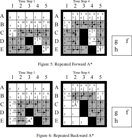
We now discuss the example search problem from Figure 2 (left) to give you data that you can use to test your implementa- tions. Figure 5 shows the first two search processes of Repeated Forward A* for the example search problem from Figure 2 (left). Figure 5 (left) shows the first A* search, and Figure 5 (right) shows the second A* search. In our example problems, A* breaks ties among cells with the same f-value in favor of cells with larger g-values and remaining ties in an identical way. All cells have their user-supplied h-values in the lower left corner, namely the Manhattan distances.  Generated cells (= cells that are or were in the open list) also have their g-values in the upper left corner and their f-values in the upper right corner.  Expanded cells (= cells that are in the closed list) are shown in grey.  (The cell of the target does not count as expanded since the A* search stops immediately before expanding it.)  The arrows represent the tree-pointers, which are necessary to identify a shortest path after the A* search.  Similarly, Figure 6 shows the first two searches of Repeated Backward A*, which searches from the target to the current cell of the agent.

5 Improving Repeated Forward A*

Adaptive A* uses A* searches to repeatedly find shortest paths in state spaces with possibly different start states but the same goal state where action costs can increase (but not decrease) by arbitrary amounts between A* searches.1   It uses its experience with earlier searches in the sequence to speed up the current A* search and run faster than Repeated Forward A*.  It first finds the shortest path from the current start state to the goal state according to the current action costs.  It then updates the h-values of the states that were expanded by this search to make them larger and thus future A* searches more focused. Adaptive A* searches from the current state of the agent to the target since the h-values estimate the goal distances with respect to a given goal state.  Thus, the goal state needs to remain unchanged, and the state of the target remains unchanged while the current state of the agent changes. Adaptive A* can handle action costs that increase over time.

To understand the principle behind Adaptive A*, assume that the action costs remain unchanged to make the description simple. Assume that the h-values are consistent. Let g(s) and f(s) denote the g-values and f-values, respectively, after an A* search from the current state of the agent to the target.  Let s denote any state expanded by the A* search.  Then, g(s) is the distance from the start state to state s since state s was expanded by the A* search. Similarly, g(sgoal ) is the distance from the start state to the goal state.  Thus, it holds that g(sgoal )  = gd(sstart ), where gd(s) is the goal distance of state s. Distances satisfy the triangle inequality:

gd(sstart )    ≤   g(s) + gd(s)

gd(sstart ) − g(s)    ≤   gd(s)

g(sgoal ) − g(s)    ≤   gd(s).

Thus, g(sgoal ) − g(s) is an admissible estimate of the goal distance of state s that can be calculated quickly. It can thus be used as a new admissible h-value of state s. Adaptive A* therefore updates the h-values by assigning:

h(s) := g(sgoal ) − g(s)

for all states s expanded by the A* search. Let hnew (s) denote the h-values after the updates.

The h-values hnew (s) have several advantages.  They are not only admissible but also consistent.  The next A* search with the h-values hnew (s) thus continues to find shortest paths without expanding states that have already been expanded by the

current A* search. Furthermore, it holds that:

f(s)    ≤   gd(sstart )

g(s) + h(s)    ≤   g(sgoal )

h(s)    ≤   g(sgoal ) − g(s)

h(s)    ≤   hnew (s)

since state s was expanded by the current A* search. Thus, the h-values hnew (s) of all expanded states s are no smaller than the immediately preceeding h-values h(s) and thus, by induction, also all previous h-values, including the user-supplied h-values. An A* search with consistent h-values h1 (s) expands no more states than an otherwise identical A* search with consistent h-values h2 (s) for the same search problem (except possibly for some states whose f-values are identical to the f-value of the goal state, a fact that we will ignore in the following) if h1 (s) ≥ h2 (s) for all states s.  Consequently, the next A* search with the h-values hnew (s) cannot expand more states than with any of the previous h-values, including the user-supplied h-values.  It therefore cannot be slower (except possibly for the small amount of runtime needed by the bookkeeping and h-value update operations), but will often expand fewer states and thus be faster.  You can read up on Adaptive A* in Koenig and Likhachev, Adaptive A* [Poster Abstract], Proceedings of the International Joint Conference on Autonomous Agents and Multiagent Systems (AAMAS), 1311-1312, 2005.

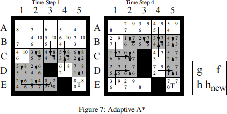
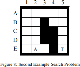
Figure 7 shows the first two searches of Adaptive A* for the example search problem from Figure 2 (left).  The number of cell expansions is smaller for Adaptive A* (20) than for Repeated Forward A* (23), demonstrating the advantage of Adaptive A* over Repeated Forward A*.  Figure 7 (left) shows the first A* search of Adaptive A*.  All cells have their h-values in the lower left corner. The goal distance of the current cell of the agent is eight. The lower right corners show the updated h-values after the h-values of all grey cells have been updated to eight minus their g-values, which makes it easy to compare them to the h-values before the h-value update in the lower left corners.  Cells D2, E1, E2 and E3 have larger h-values than their Manhattan distances to the target, that is, the user-supplied h-values. Figure 7 (right) shows the second A* search of Adaptive A*, where Adaptive A* expands three cells (namely, cells E1, E2 and E3) fewer than Repeated Forward A*, as shown in Figure 5 (right).

6 Questions

Part 0 - Setup your Environments [10 points]: You will perform all your experiments in the same 50 gridworlds of size 101 × 101. You first need to generate these environments. To do so, give each tile in the gridworld a 30% chance of being blocked, and a 70% chance of being unblocked. Then, use one of the search algorithms we discussed in class to verify that there exists a path from the top left of the grid to the bottom right.  If the path exists, add it to the set of 50 gridworlds. Otherwise, generate a new random gridworld.

In your report, explain what method you chose to use to check for the existence of a path.  Justify your choice, and whether you think your selection is the fastest way to check if a path exists. If you didn’t implement the most efficient way to check for the existence of a path, what do you think would be the most efficient?

Part 1 - Understanding the methods [10 points]: Read the chapter in your textbook on uninformed and informed (heuristic) search and then read the project description again.  Make sure that you understand A* and the concepts of admissible and consistent h-values.

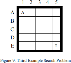
a) Explain in your report why the first move of the agent for the example search problem from Figure 8 is to the east rather than the north given that the agent does not know initially which cells are blocked.

b) This project argues that the agent is guaranteed to reach the target if it is not separated from it by blocked cells. Give a convincing argument that the agent infinite gridworlds indeed either reaches the target or discovers that this is impossible infinite time. Prove that the number of moves of the agent until it reaches the target or discovers that this is impossible is bounded from above by the number of unblocked cells squared.

Part 2 - The Effects of Ties [15 points]: Repeated Forward A* needs to break ties to decide which cell to expand next if several cells have the same smallest f-value.  It can either break ties in favor of cells with smaller g-values or in favor of cells with larger g-values. Implement and compare both versions of Repeated Forward A* with respect to the number of expanded cells. Explain your observations in detail, that is, explain what you observed and give a reason for the observation.

[Hint: For the implementation part, the simplest thing to do is to store both the f and g values, and then define a comparison operator that first checks the f value and then secondly checks the g value in case of a tie.  So for instance, if we were breaking ties in favor of smaller g values, we would have (f : 5, g : 3) < (f : 6, g : 3) and (f : 5, g : 3) < (f : 5, g : 2). However, if your language’s heap implementation does not allow you to set your own comparison operator, you can do this by multiplying g by a number very slightly less than 1, so that f = 0.9999g + h or something similar. This biases the priority queue to push large g values to the top over large h values. This ties into what we talked about in class, where breaking ties in favor of smaller heuristics is effectively like making the heuristics a tiny bit larger when calculating f. For the explanation part, consider which cells both versions of Repeated Forward A* expand for the example search problem from Figure 9.]