闪电代写 -代写CS作业_CS代写_Finance代写_Economic代写_Statistics代写_代码代做_IT代写_加急帮助

Hello, dear friend, you can consult us at any time if you have any questions, add WeChat: daixieit

Assignment 2

Task 1

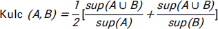
In this task we need to write a function to return Kulczynski measure. The Kulczynski measure is defined as:

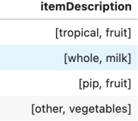
The Groceries dataset is selected for itemsets, it contains 38765 rows for Market Basket Analysis. Some data samples are as follows:

In Kulczynski funciton, we need to calculate the support for A, B, A and B. The function code is as follows:

import pandas aspd

import numpy as np

def kulczynski(iterm_sets, rule):

rule a part, rule b part = rule

support a = sum(groceries_data['itemDescriptionapply(

lambda x : len(set(x)&set(rule a part)

)== len(rule a part)

support b= sum(groceries_data['itemDescriptionapply(

lambda x : len(set(x)&set(rule b part)

)== len(rule b part)

support a and b= sum(groceries_data['itemDescriptionapply(

lambda x : len(set(x)&set(rule a part+ rule b part)

)== len(rule a part+ rule b part)

return(support a and b/support a + support a and b/support b)*

0.5

Task 2

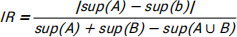
In this task we need to write a function to return imbalance ratio. The imbalance ratio is defined as:

The Groceries dataset is selected for itemsets. In imbalance ratio funciton, we need to calculate the support for A, B, A and B. The function code is as follows:

import pandas aspd

import numpy as np

def imbalance_ratio(iterm_sets, rule):

rule a part, rule b part = rule

support a = sum(groceries_data['itemDescriptionapply(

lambda x : len(set(x)&set(rule a part)

)== len(rule a part)

support b= sum(groceries_data['itemDescriptionapply(

lambda x : len(set(x)&set(rule b part)

)== len(rule b part)

support a and b= sum(groceries_data['itemDescriptionapply(

lambda x : len(set(x)&set(rule a part+ rule b part) )== len(rule a part+ rule b part)

return np.abs(support a - support b) / (support a + support b - support a and b)

Task 3

Excluding the case of a single item, there contiains (N-1)! possible valid itemsets.

Task 4

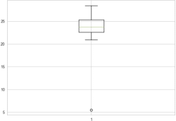
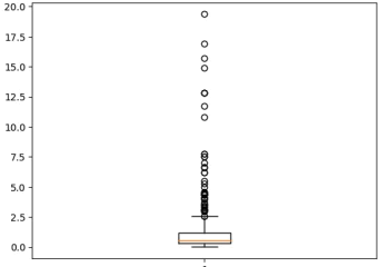
Through the box plot we can determine the outlier, the outlier is 5.49. The boxplot regards outliers as points in the outer 1% of a normal population.

Task 5

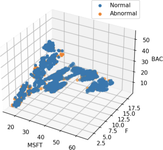
After reading the dataset, the percentage of changes was calculated, and a one-class SVM classifier was used to identify outliers. The 3D scatterplot of the dataset with object is color-coded outlier is shown in the figure below.

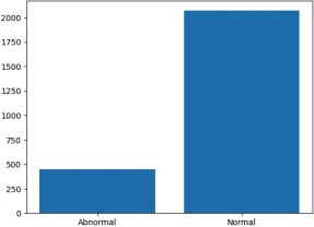
The histogram and the frequencies of the abnormal detection results are shown in the figure below, in which 18% of the samples are abnormal samples. The results of One-class SVM are not based on distance and density, from distance.

import pandas aspd

#Load CSVfile, setthe 'Date'values asthe index ofeach row, anddisplay the first rows ofthe dataframe

stocks = pd.read excel('stocks.xlsx header='infer')

stocks.index = stocks['Date]'

stocks = stocks.drop(['Dateaxis=1)

N,d= stocks.shape

delta = pd.DataFrame(

100*np.divide(stocks.iloc[1:,:].values-stocks.iloc[:N-1,:].values, stocks.iloc[:N-1,:].values),

columns=stocks.columns, index=stocks.iloc[1:].index

)

delta.head()

from sklearn.svm import OneClassSVM

ee = OneClassSVM(nu=0.01, gamma='auto')

yhat = ee.fit predict(delta)

import matplotlib.pyplot asplt

fig = plt.figure(dpi=150)

ax = fig.add subplot(projection='3d')

ax.scater(stocks['MSFTiloc[np.where(yhat==1)[0]+ 1],

stocks['Filoc[np.where(yhat==1)[0]+ 1],

stocks['BACiloc[np.where(yhat==1)[0]+ 1])

ax.scater(stocks['MSFTiloc[np.where(yhat==-1)[0]+ 1],

stocks['Filoc[np.where(yhat==-1)[0]+ 1],

stocks['BACiloc[np.where(yhat==-1)[0]+ 1])

plt.legend(['Normal 'Abnormal]')

ax.set xlabel('MSFT')

ax.set ylabel('F')

ax.set zlabel('BAC')

Task 6

The data set is first subjected to PCA dimensionality reduction, and then the distance of each sample is obtained by nearest neighbor calculation. We plotted the sample distances as boxplots. As shown in the figure below, samples with a sample distance greater than 2.5 can be regarded as outliers.

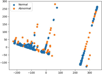
The scatter diagram of PCA is shown in the figure below. It can be seen that the distance between the outlier point and other points is relatively long.

df= pd.read csv(url, header=None)

data = df.values

X, y = data[:, :-1], data[:, -1]

from sklearn.decomposition import PCA

pca = PCA(n_components=2)

X pca = pca.fittransform(X)

from sklearn.neighbors import NearestNeighbors

knn = NearestNeighbors(n_neighbors=2)

knn.fit(X pca)

plt.scater(X pca[distances.mean(1)<2.5, 0], X pca[distances.mean(1)<2.5, 1])

plt.scater(X pca[distances.mean(1)>2.5, 0], X pca[distances.mean(1)>2.5, 1])

plt.legend(['Normal 'Abnormal]')

Task 7

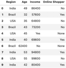
There are many HTML tags in the web page, such as html, body, h1, p, table, thead, tr, th, rd. By consulting the introduction of the HTML web page, the meaning of each tag is as follows:

. html, page start and end

. body, content start and end

. h1, header

. p, paragraph

. table, table start and end

. thead, header of table

. tr, row of table

. th, head row of table

. td, content row of table

With Beautiful Soup, data is crawled and stored in tables. The result is shown in the figure below.

from bs4import BeautifulSoup

data =

BeautifulSoup(requests.get('htp:/eecs.qmul.ac.uk/~emmanouilb/income _table.htmltext)

header = [x.text.strip()for x in table.find al(t'head')[0].find al(t'h')]

table = data.find(t'able')

table_body = table.find(t'body')

rows = table_body.find al(t'r')

table_data = []

for row in rows:

cols = row.find al(t'd')

cols = [ele.text.strip()for ele in cols]

table_data.append([ele for ele in cols ifele])

table_data = pd.DataFrame(table_data, columns=header)

Task 8

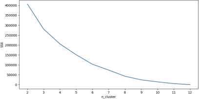
Through Beautiful Soup, we crawl webpages with multiple keywords. And the frequency of words in the article is counted, and then the web pages are clustered. We experimented with various numbers of clusters and recorded the clustering loss. The elbow diagram is shown in the figure below. It can be seen from the figure that the optimal number of clusters is 6.