1    Introduction to Python

1.1    Background

Python is a general purpose programming language and is completely free.  It is not specifically designed for analyzing data, but it has become one of the most popular platform for data science as well as artificial intelligence.

Since its birth,  so many people have contributed to Python that almost any mathematical and statistical task that you can imagine has probably been implemented in Python.  Therefore, per- forming mathematical computations and data analysis is more of an art of finding what existing tools for your task than a challenge of implementing the task yourself.

Also, because so many people have contributed to Python, the universe of Python tools has become huge. Therefore, neither of the following two is usually a good idea:

•  Download every existing Python tool to your computer.

•  Load all tools installed in your computer into the memory when you launch Python.

Meanwhile,  it  is  silly to try  and  download  individual tools  one  by  one.   To  address this  issue, tools that serve related purposes have been organized into toolkits called libraries.  For example, all linear algebraic tools are contained in the library called NumPy, a library that we will use all the time.  Most of the statistical tools that we will use in this course are contained in pandas and statsmodels libraries. Also, SciPy contains many other useful mathematical tools like optimisation and numerical equation solvers.

Therefore,  we  will  need  several  different  libraries  for  performing  forecasting  and  perhaps  other kinds of economic analysis. Even though it is possible to install the libraries one by one, it is more convenient to install all of them once and for all; this is achieved by installing the free data science platform Anaconda on your computer.

If you try to load all libraries provided by Anaconda into memory when lauching Python, it would probably take forever to launch it.  Therefore, we only load a library into Python when needed. This leads to the first important command in Python:  import.  This command loads the named library into memory so that it may be used later on. For example, the following commmand loads NumPy into the memory.  It is very standard to use a shorthand “np” for NumPy, so we append “as np” to the command so that the library will be referred to as np later.

[1]:  import numpy as np

1.2    Task 1:  Multiplying Matrices

Now that we  have  loaded  NumPy  into  memory,  we  may  start  doing  some  linear  algebra  using Python. Let us try multiplying the following two matrices together:

A =  (3(2)

B =  (3(6)

1) .

8    1) .

Of course, we need to create these two matrices first using NumPy.  NumPy provides a command for creating a matrix and it is named non-creatively as matrix.  Executing a command is referred to as a call of the said command. For this reason, a command is also referred to a callable. Following standard  convention  in  the  computer  science  literature,  such  a  callable  is  also  referred  to  as  a function.   However,  a  “function” in the context of programming language is somewhat different from a “function” in mathematics.  In order to call this command, we use the syntax np.matrix, which says that we are calling the matrix command within the library np (which is our nickname for NumPy).

NumPy supports several different ways to create a matrix.  In order to learn about them, you can simply type “numpy create matrix” in your favorite search engine and probably land in this manual page.  This may seem daunting, but over time you will feel more and more comfortable reading manual pages like this.  For now, we only need the simplest possible way to create a matrix, by specifying its entries.  NumPy has a very specific way of defining matrices: we specify its entries row by row, and each row is enclosed with a bracket; the entire matrix is also enclosed with a bracket. The right hand side of the first line in the next block defines the matrix A.

Just like in mathematics, we want to give a name to our newly created matrix.  This is achieved by the equal sign command in Python.   This command is very different from what it means in mathematics.   It is not an assertion that the two sides are equal; that purpose is served by the operator ==.  The equal sign command simply says that we give the right hand side a name, and the name is the symbol on the left hand side.  Therefore, the first line of the following block first creates a new matrix and then give it a name, A.

Warning:   it  is  usually  a  very  bad  idea  to  name  your  objects  by  A,  B,  x  or  y.   This  practice makes it very difficult for you to read your code later on and figure out what it is trying to do. You should  develop a good habit of giving long and  descriptive names to your objects such as Jacobian__of_cost__function so that you (and other developers) can read and understand your code later on.

[2]: A = np.matrix([[2, 4], [3, 1]]);

B = np.matrix([[6, 9, 3], [3, 8, 1]]);

At this point, you may be tempted to run A * B. This will lead to the correct result, but I do not recommend it.  If you defined A and B as arrays instead of matrices, the star operator will attempt to multiply the two arrays entry by entry and return an error because the two arrays are of different sizes.  Matrix multiplication is implemented by the callable matmul in NumPy and it is safer to call this function instead.  After we compute the matrix product, we give the product a name, A__times__B. Therefore, the right hand side of the first line creates an unnamed object which is the matrix product of A and B and then the equal sign command names that object C. Finally we print out the result.

[3]: A_times_B = np .matmul(A, B);

print("The product between A and B is ");

print(A_times_B);

The product between A and B is

[[24 50 10]

[21 35 10]]

The following code demonstrates the difference between A * B and np.matmul(A, B). If you find it confusing, you can ignore it for now as long as you remember using np.matmul to perform matrix multiplication.  Whenever the Python interpreter (called the kernal) sees the sharp sign #, it will ignore the rest of the line.  Texts following the sharp sign are called comments; they are ignored by the kernel but help readers understand what the code is trying to do.

[4]: A_star_B = A * B;  # I do not recommend this but it happens to yield the␣

↪ correct result.

print("A * B is ");

print(A_star_B);

A_array = np .array([[2, 4], [3, 1]]);    # now A and B will be defined as arrays.

B_array = np .array([[6, 9, 3], [3, 8, 1]]);

A_times B array = np .matmul(A_array, B_array);

print("The matrix product of A and B as arrays is ");

print(A_times B array);   # same result as before; this is robust programming.

# The following line will yield an error. If you are not convinced, uncomment␣ ↪ it and run the block.

# A_star B array = A_array * B_array

A * B is

[[24 50 10]

[21 35 10]]

The matrix product of A and B as arrays is

[[24 50 10]

[21 35 10]]

1.3    Task 2:  Computing Roots of a Polynomial

In this task, we try to compute all the (complex) roots of the following polynomial:

f() = 2 3 − 5 2 + 3 + 6.

We do not know yet how to compute the roots of a polynomial in Python.  We do not even know how to represent a polynomial. However, we have high hope that Python already contains a method for doing that. Therefore, we search for “python polynomial roots” in any search engine.

[5]:  # I don't know yet how to compute the roots of a polynomial

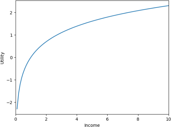
1.4    Task 3:  Plotting the Graph of Logarithm

In this task, we learn the important concept of objects in Python.

In general, to plot the graph of a known function, we sample finitely many points on the graph hoping that connecting those points with a smooth curve would give us a good representation of the true graph, which consists of infinitely many points in theory.  This strategy usually works unless your function is very ugly. Here we know as a fact that logarithm is a smooth function.

The way we sample the points on the graph is to first create finitely points in the domain of the function (the set of positive real numbers) and then compute the value of the function at each point. NumPy provides us with a useful function linspace which creates equally spaced sample points in the given range:  np.linspace(a, b, n) creates n equally spaced points between a and b (inclusive). Finally, as a general purposse programming language, Python itself does not define the logarithm function; this function is also provided by NumPy.

Warning.   Of ocurse, NumPy also provides the exponential function.   However, when you apply it to a square matrix, it computes the exponential of each individual entry instead of the matrix exponential.

[6]: log_graph_x = np.linspace(.1, 10, 100);

log_graph_y = np.log(log_graph_x);

Plotting is handled by the python library called matplotlib. This library provides an object called pyplot, which we will use to generate our plot.

Before starting to work with pyplot, we will briefly talk about what objects are. It may be help to draw an analogue with an object in daily life, a car.  A car is a complicated machine.  It contains many internal parts and they have to work together in a particular way so that the car can move forward.  Unless you are (or want to become) a car mechanic, you do not care about any of these internal parts. What you care about is how to operate a car. For example, you want to know how to star, accelerate, or decelerate your car and how to make it turn left or right.  Sometimes, you also want to learn the status of your car such as it current speed and the amount of fuel in its tank.

The situation is very similar in the Python world.  An object is something in the Python world that you can interact with.  For the object to do something it is supposed to do, it needs to store some information in the computer’s memory, but that hardly concerns you. What you really care about is what the object can do for you:  whether you can turn the object left and right or flip it.  Each trick the object can perform for you is called a method.  Sometimes you want to know that status of your object, and such a status is called a attribute.  The syntax for obtaining a particular attribute is object.attribute, and the syntax for calling a particular method is object.method(parameters). For example, if the object in question is my red hatchback, then the following two lines should make sense.

•  my__red__hatchback.speed()

•  my__red__hatchback.turn__right(90) # turning right by 90 degrees.

Coming back to the task at hand, our pyplot object (or plt in its standard nickname) is a canvas that allows us to draw figures on it.  As mentioned above, we do not care about what information this object stores in the computer memory or how exactly it draws things.  What we care about is what it can draw.   In the current task,  we simply draw the graph of our logarithm function using the sample points that have been generated, and then we create the labels of the axes.  Let us imagine that this logarithm function is actually a consumer’s utility index, so we will label the horizontal axis as income and the vertical axis as utility.  The manual page of pyplot has a complete list of what parameters each method takes, but usually we only need first first few.  For examples, the most important parameter to the plot method are the x values and the y values.

Finally, after we draw everything we want, we can either show the canvas on the computer screen with plt.show(), or save the figure in some file using plt.savefig(‘file path’).

Before we close this section, I want to mention the concept of class.  There is an abstract notion of “car” which refers to a specific type of motor vehicles instead of any particular car.   My red hatchback or Thomas’s blue sedan are all particular instances of this abstract notion of car.  In the Python world, the abstract notion is called a class, and each particular instance is an object.  For example, my red hatchback is an object of the class of car. The class specifies the minimum things that each object should do, like showing its current speed and turning right by any degrees.

[7]: import matplotlib.pyplot as plt;

plt .plot(log_graph_x,log_graph_y);

plt .xlim([0, 10]);      # Find what this line means through the manual page of␣

↪pyplot.

plt .xlabel( 'Income ');

plt .ylabel( 'Utility ');

plt .show();

# plt.savefig('log_utility.eps')

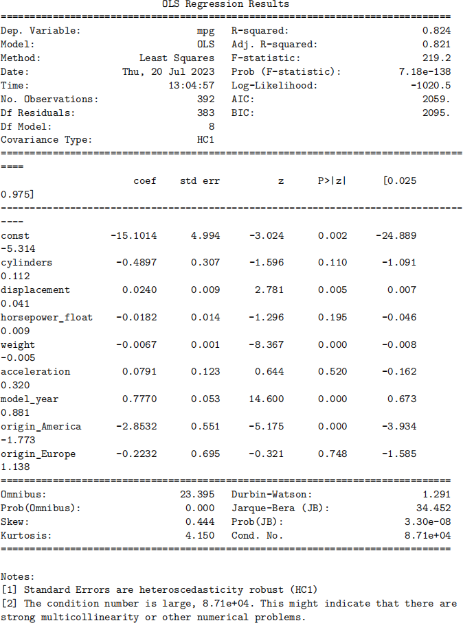
1.5    Task 4:  What Determines a Car’s Fuel Efficiency?

In this task, we will run an OLS regression using the Python library statsmodels. The data set we use is a standard one: mpg (miles per gallon of gasoline) by cars sold in the US market with model years between 1970 and 1982. The data file can be downloaded here.

The Python library pandas provides methods for importing data from various formats.   In this case, our data are in plain texts, and different columns are separate by one or more spaces.  It turns out that the correct method for importing this format is pd.read__table.  The file itself does not contain names of the columns, but an companion file does; we give the columns names according to that companion file “auto-mpg.names” in the original zip file.  If we look at the manual page of pandas.read__table, this method can take dozens of parameters.  It is impossible for anybody to remember the order in which the parameters should be presented.  Therefore, a better way is to specify the names of the parameters we will supply.  The first parameter of read__table is always the path of the data tile  (and hopefully it is not too difficult to remember this).  We supply two additional parameters:  “sep” specifies what separate columns of our data  (one or more spaces in this case) and “names” specifies the names of the columns.

The read__table method  (and all other similar methods in pandas) creates an object of the class DataFrame. The second line in the following cell gives a name mpg__data to this object.  All entries in the same column are supposed to have the same data type.  If it appears that contents of the same column are of different types, Python will play it safe and treat them as strings instead of numbers. After we load data into the memory, we should check that the data types are all correct by printing out the dtypes attribute of our DataFrame.

Here we need to be falimiar with some Python jargons.  “float64” means a real number,  “int64” means an integer, and “object” means a generic object and string in the current context.  It is a  bit weird that horsepower is of type “object” instead of “float64”.  Inspecting the original data set  reveals that this is because this field is missing for some car models and a question mark is placed  there.  What we do next is to convert the column to the “float64” type using the method astype.  However, a naive application of the method will generate an error because it cannot convert “?”  to  a real number.  The solution is to first replace every appearance of “?”  with “nan” (meaning “not  a number”) before doing the conversion.

The  “origin”  column  of the  data  set  denotes the  origin  of the  card,  where  1  denotes  America, 2 denotes Europe and 3 denotes Asia.  In order to determine whether the origin affects the fuel efficiency of a car,  we need to generate dummy variables of the origin.   You are encouraged to search for a method that does this before reading on.   It turns out that this is achieved by the get__dummies function provided by pandas.

The next step is to insert the three new columns (horsepower__converted and two of the three origin dummies created) into the data frame.  This is achieved by the assign method of our DataFrame object.   What is a bit counterintuitive is that this method does not simply expand the existing object.  Instead, it creates a new DataFrame containing all the old columns and the newly added column.   The right hand side of the fifth line of the following cell creates that new DataFrame (without modifying mpg__data) and then name the new DataFrame mpg__data__complete.

[8]: import pandas as pd

mpg_col_names = [ 'mpg ', 'cylinders ', 'displacement ', 'horsepower ', 'weight ',␣ ↪ 'acceleration ', 'model_year ', 'origin ', 'car_name '];

mpg_data = pd .read_table( 'auto-mpg.data ', sep = '\s+ ', names = mpg_col_names);

print(mpg_data .dtypes)

mpg_horsepower = mpg_data[ 'horsepower '];  # the right hand side creates a new␣

↪DataFrame consisting of the single column names  'horsepower' of mpg_data # this next line will generate an error:

# mpg_horsepower.as type('float64')

horsepower_converted = mpg_horsepower .replace( '? ', 'nan ') .astype( 'float64 ');

origin_dummies = pd .get_dummies(mpg_data[ 'origin ']);

origin_dummies .columns = [ 'Am ', 'Eu ', 'As '];     # we rename the columns of the␣

↪ three columns of origin_dummies

mpg_data_complete = mpg_data .assign(horsepower_float = horsepower_converted,␣

↪origin_America = origin_dummies[ 'Am '], origin_Europe = origin_dummies[ 'Eu ']);

print(mpg_data_complete .dtypes)

mpg

cylinders

displacement

horsepower

weight

acceleration

model_year

origin

car_name

dtype: object

mpg

cylinders

displacement

horsepower

float64

int64

float64

object

float64

float64

int64

int64

object

float64

int64

float64

object

weight

acceleration

model_year

origin

car_name

horsepower_float

origin_America

origin_Europe

dtype: object

float64

float64

int64

int64

object

float64

uint8

uint8

Essentially, what we have been doing is preprocessing our data.  This looks cumbersome and boring, but is necessary.  Data obtained from real world sources are rarely as neat as those contained in the CDs attached to econometric textbooks. Preprocessing data is an essential skill in data analysis.

Now that we have generated all the columns we need, we will create our OLS model.  The OLS

regression model along with many other essential tools for time series analysis and forecasting are contained in the Python library statsmodels.  For what we plan to do, it will be convenient to creat a new DataFrame consisting only of the independent variables that we will use in the regression. We do this using the double bracket method of DataFrame:  single bracket allows us to select one column,  while  double  bracket  allows  us to  select  multiple  columns.   Note that  statsmodels  has a convenient method add__constant which will add a constant column to our list of independent variables.

The way statsmodels works, which is also the way many other similar data analytical tools work, may  seem  a  bit  counterintuitive.   It  does  not  provide  a  function  that  runs  an  OLS  regression. Instead, it treats an OLS model as an object.  The right hand side of the fourth line of the next cell creates this OLS model object and then we name it as mpg__OLS__model; the “missing” parameter specifies what to do with observations (rows) containing missing values (such as those rows with missing horsepower values) and our choice is to drop those observations for simplicity. Recall that an object is essentially a toy you can play with.  Besides finding the least square estimator of the model, this object allows you to do many other things.  If interested, the reader is encouraged to browse its manual page. We will come back to some of those other methods later in the course.

For now, we will simply make a least square estimator of our model using the fit method.  Since we have all taken introductory econometrics, we know that it is better to use heteroskedasticity-robust covariance matrices, which is obtained by specifying cov__type as “HC1” in fitting the model.  This method generates an object of the class RegressionResults. Finally, we can print out the summary of our regression model by using the summary method of the result object.

In this task, we learned how to import data from a file, some basic preprocessing of data and how to fit an OLS model using statsmodels.  We worked with several objects during the process.  This is common place in Python. For every object, we do not ask “what the object looks like” or “what is inside the object”; instead, we ask “how I can interact with the object” and “what the object can do for us”. This is a very important principle to keep in mind.

Exercise: for the OLS model we just fit, perform a Wald test on the joint significance of cylinders, displacement, and horsepower__float.

[9]: import statsmodels.api as sm

mpg_indep_variables = mpg_data_complete[[ 'cylinders ', 'displacement ',␣ ↪ 'horsepower_float ', 'weight ', 'acceleration ', 'model_year ',␣

↪ 'origin_America ', 'origin_Europe ']];

indep_names = mpg_indep_variables .columns;

num_cols = indep_names[:len(indep_names) - 2];

print(num_cols);

# mpg_indep_variables.loc[:, num_cols] = (mpg_indep_variables.loc[:, num_cols]␣

↪ - mpg_indep_variables.loc[:, num_cols].mean()) / mpg_indep_variables.loc[:,␣ ↪ num_cols].std();

mpg_indep_variables = sm .add_constant(mpg_indep_variables);

mpg_OLS_model = sm .OLS(mpg_data[ 'mpg '], mpg_indep_variables, missing = 'drop ');

mpg_OLS_fit_result = mpg_OLS_model .fit(cov_type = 'HC1 ');

print(mpg_OLS_fit_result .summary());

Index(['cylinders', 'displacement', 'horsepower_float', 'weight', 'acceleration', 'model_year'],