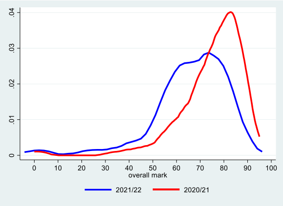
The figure below shows the distribution of the overall mark between the 2020/21 and 2021/22 cohorts.  In  2020/21 the  mean  (standard  deviation) was  75%  (14%),  compared to a  mean (standard deviation) of 66% (16%) in 2021/22. Clearly, there has been a leftward shift in the mark distribution despite all elements of the assessment being open book. The marks have moved towards that of the pre-pandemic distribution, i.e. the mean (standard deviation) of the 2019/20 cohort where the assessment was 100% unseen examination was 56% (18%).

3. Commentary

Comments on analysis of grades:

The  coursework  element   (2)  covered  basic  econometrics  and  the  violation  of  classical assumptions. This component of the assessment comprised two questions both compulsory where the second was a short Stata assignment. The examination (3) again was based on two compulsory questions covering micro- and macro-econometrics respectively.

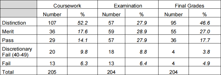
Student performance in all components of assessment was excellent approximately 52% (28%) gained a distinction in the coursework (examination). With regard to the overall marks 47% gained a distinction with 27% obtaining a merit. This was despite making the coursework and examination more challenging than in 2020/21 in order to stretch the students and differentiate at the upper end of the distribution.

Those students who obtained a grade of 40% or below in any elements of the assessment will have to retake the appropriate component in the August resit period. For the coursework and exam this comprised 6.3% and 6.4% of students respectively, where only 2 students had less than the 40% threshold for both elements of assessment.

Comments on student performance in the main elements of assessment:

Coursework

In question 1 the majority of students lost marks in part (i) where they needed to explain in detail how to test for differential profits and sales elasticities across the different age groups. The answer was worth 25% and should have specified that restricted least squares needed to be used to undertake a joint test of sales and profits differential age elasticities. Other common mistakes which lead to marks being lost in question 1 were: not stating holding other things constant or ceteris paribus when interpreting parameter estimates; incorrectly set up the null hypothesis, and; not correctly introducing interactive effects into original model between profit and age dummies, and sales and age dummies, in order to allow for differential profit and sales elasticities with respect to age (part h).

In question 2 which contained the Stata assignment the majority of marks on average were lost in parts (d) and (e) both worth 30%, where the White test needed to be undertaken and then a test for autocorrelation in the presence of a lagged dependent variable respectively. Marks were lost in both parts for not explicitly providing the null and alternative hypothesis tested, or not giving  the  appropriate  critical  value.  Some  students  used  the  inbuilt  “imtest”  to  test  for heteroscedasticity which the question explicitly stated not to do, rather the test statistic should have been calculated by hand in the Stata *.do file. In part (e) some students used a standard durbin-watson statistic rather than the durbin h-statistic which should be used in the presence of a lagged dependent variable, or failed to realise that the test statistic is normally distributed. Other common mistakes were: decimal place and unit errors in interpretation; not stating ceteris paribus when  interpreting  parameter estimates;  not  calculating tax and  income elasticities, where the estimates from part (a) and the sample means needed to be used in order to construct elasticity  (not transformation the  model  into  a  log-log  specification  as  some students did); obtaining incorrect critical values for durbin-watson statistic, and; not randomising the data as required using the function “set seed” .

Examination

Question  1  focused on  micro-econometrics whilst  question 2 was  on  macro-econometrics. Common mistakes and errors across both questions were one or more of the following: not fully stating the null and alternative hypotheses; using incorrect test statistics, and; not providing the correct critical value.

Question  1  provided  students  with  Stata  output  from  modelling  the  saving  behaviour  of individuals using UK cross sectional data for 2017 from Understanding Society. Part (a) focused upon the likelihood of saving from a logit specification requiring students to calculate marginal effects at the mean from the given coefficients , and then interpret the marginal effects. The answers to this part were in general excellent, and marks were generally only lost for rounding errors, decimal place errors, incorrect units in interpretation, or not stating ceteris paribus. In part (b) students were provided with Stata output from modelling the amount of savings using a tobit estimator with censoring on zero savings. They were required to calculate the predicted monthly savings for an individual with given characteristics and then calculate the probability that the individual saved between £10 and £1,000 per month. The most common mistake here was to use base 10 instead of the natural logarithm, the units that savings entered the regression equation, or not being able to calculate the associated probability from the normal distribution.

In the final part of question 1 - part (c) - savings were modelled via a Heckman sampleselection estimator. Students were generally good at explaining the inverse Mills ratio, in terms of the direction of bias in OLS and statistical significance (part c(i)). However, for part (c(ii)) only a small minority of students were able to explain how you could use the estimates from the treatment equation to proxy the coefficients found from the Logit model in part (a). In part (c(iii)) there were errors in explaining how the model is identified, and the implicit assumption that working in the financial sector and/or having good health only influence the treatment, i.e. probability of saving, not the outcome, i.e. the amount saved. If this assumption is not met then identification is only through non-linearity, which only a small number of students stated. The majority of students were unable to state precisely the hypothesis tested by the Wald statistic in part (c(iv)), either not specifying hypothesis tested correctly and/or not explicitly stating that the statistic is a joint test of the parameters in the outcome equation.

In question 2 students were given Stata output from modelling the demand for money as a function of GDP using quarterly seasonally adjusted data from 1997q1 to 2020q4. The output included ADF tests for each series in log levels and first differences, and ADF tests on the OLS residual. Stata output was also provided on a forecast of the demand for money, where two alternative models were estimated over the period 2010q1 through to 2020q4: an ARIMA(1,0,1) and an ARIMA(2,0,1). Students were asked to write a small report based upon the Stata output provided. To provide some guidance and also mark allocation, students were told that the discussion should be based around: (a) an assessment of the OLS regression and the time series  properties  of  the  data  from  the  ADF  tests  provided,  including  whether  a  long-run relationship exists between the variables; (b) an examination of the two alternative ARIMA models and explanation of which specification is preferred; and (c) an explanation of any further analysis worth undertaking stating the reason why. Marks were lost in part (a) for: providing no interpretation of OLS results; not mentioning or explaining why OLS might be spurious. In terms of the ADF tests - not explicitly stating the hypothesis tested; use of incorrect critical values (e.g. including a time trend); not providing enough detail on cointegration tests, and; using same critical value rather than E-G specific values. For part (b) marks were lost for: not commenting on invertibility and/or stationarity based upon the regression output of the ARIMA models; not mentioning the role of the Q-statistic, the hypothesis tested, or critical value; not focusing explicitly on the Information Criteria and/or RMSE and the appropriate decision. A number of students did not address part (c). To gain marks here I was looking for at least two of the following: an alternative unit root test, based upon KPSS; discussion of the importance of lag length on ADF tests and optimal lag selection; inclusion of a trend term in ADF tests; use of the ACF/PACF for identifying the structure of ARIMA models, or; the Johansen approach to cointegration if there are more than two variables in system (along with the disadvantages of the E-G approach to cointegration).

What aspects of the module do you feel were successful this year?

In 2021/22 both problems and Stata questions were posted and answers provided with a two week lag. Despite this a good number of students submitted their answers and were able to gain timely feedback on their work (usually within 2 working days). Whilst some students were based in Sheffield and so had face-to-face Stata computer practicals, there were ten weekly one hour Collaborate sessions provided to cover: Stata practicals for those students not in Sheffield; questions arising from the lecture videos; and problem sets. I think these worked really well although students were less interactive than the 2020/21 cohort, perhaps due to many being based in Sheffield and so having the advantage of been able to ask questions during (or at the end) of the lecture. The student engagement activity for the module comprised four multiple choice quizzes which also seemed to work well and enabled students to obtain direct feedback on their knowledge. In summary all students arguably had more opportunities than in previous pre-pandemic cohorts to gain detailed feedback on their work at each point in the module (this is reflected in the Tell US scores below).

4. Student Module Survey Feedback

Please reflect on the response rate achieved and actions taken to promote completion of the Tell US survey for this module:

The response rate was 40.8% (87/213 students) down on last years’ rate of 48.6%. Students were asked on multiple occasions in both lectures and during the online Collaborate sessions to complete the Tell US survey. One reason for the lower response rate might have been due to the fact that I did not offer a revision session as I had done for the 2020/21 cohort. In 2020/21 the revision session was just prior to the cut-off date of the Tell US survey completion window and so a number of responses could have come in then.

Please provide a summary of:

(i)       The positive aspects in the student feedback

All summary scores were above the economics departmental average:

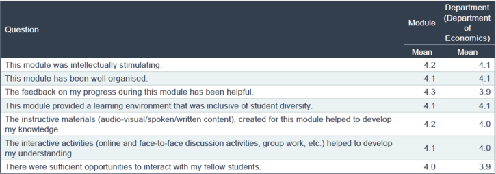
For example, proportions indicating definitely agree/strongly agree that:

- “explained the material well = 88.5%”;

-     “this module was intellectually stimulating = 85. 1%”;

-     “this module has been well organised = 86.2%”

-     “The instructive materials (audio-visual/spoken/written content), created for this module helped to develop my knowledge = 89.7%”;

-     “The feedback on my progress during this module has been helpful = 87.4%”;

-     “The interactive activities (online and face-to-face discussion activities, group work, etc.) helped to develop my understanding = 86.2%”

The feedback mark is good to see, and upon last year, which is pleasing given the effort that has gone in to create timely feedback opportunities both in the MCQs and coursework, as well as students having the option of handing in problem sets and Stata practicals in order to have these marked.

(ii)      Areas for development (if any)

NA

Please use this space to provide additional information about how you plan to respond to any issues raised in the module survey feedback.

-    To slow down the teaching pace and spend more time on explaining key concepts, whilst conversely other students thought the  pace was too  slow.  Given  such  a  large  and heterogeneous cohort in terms of background (and ability) it was difficult to pitch at a pace to please everyone.

-    Spend more time on micro- and macro-econometric topics. I agree that ideally this would be the case. However, the intake of students is from a varied background, where some will have done econometrics at undergraduate level (in years 2 and 3, e.g. Sheffield BSc students) and so should be comfortable with Topics 1-5, whilst others will have limited knowledge  of  econometrics  with  just   basic  statistical  training  and  knowledge  of regression. Hence ECN6540 gives a broad grounding in econometrics before students can specialise and go on to study micro- and/or macro-econometrics (Topics 6-9) in greater depth in the second semester.

-    There were a couple of requests for more Stata practicals. All Sheffield based students had five face-to-face Stata sessions. Given this and the fact that I also went through Stata in the online Collaborate sessions I think that there is no need for more practicals and Stata practice as students should be doing this in their own time (see PG handbook).

-    In one of the text responses for how the module could be improved it was suggested that there should be some mention or link to the dissertation at the end of the academic year. This is a good idea. I do this in the introductory lecture at the start of the semester reiterating that students will need to use Stata for their dissertation, but in future it would be worth reminding students on more occasions in order to encourage them invest in learning the software early on (although the coursework forces this and should help the dissertations).

-    A couple of students suggested making the lectures more interactive. This was tricky for this cohort given some were being taught face-to-face whilst others were remote learning via a live transmission. In previous years I have made use of clicker questions and again this  might  be  worth  considering  in  the  future,  although  MCQs  are  heavily  used  for engagement tasks.

If applicable, please indicate, what other changes you intend to implement next year:

I intend keeping the assessment the same. However, if the examination is online then rather than having 24 hours to complete the exam I would move into line with other modules and use a 2 ½ online exam window.