EViews Part

Background

The purpose of this project is to analyze the predictability of the Dow Jones Industrial Average index returns.

The project would be easier to handle in EViews, as it involves importing and manipulating the data. You

will need to estimate and interpret the models, tests the main assumptions and propose strategies to address any arising statistical issue.

Task 1

The Excel spreadsheet “DOW_Dataset.xlsx” contains the data for the task. The dataset contains the time series of (i) the Dow Jones Industrial Average index prices (DOW), (ii) the S&P 500 implied volatility index (VIX), (iii) the USD-GBP exchange rate as U.S. Dollars to one U.K. Pound Sterling (USDGBP), and (iv) the crude oil prices from the West Texas Intermediate (OIL). All the time series are downloaded from FRED. The dataset time period is from 02 January 2013 to 29 July 2022, at a daily frequency.

1. Compute the log market returns on the Dow Jones (denote it as DOWret) and plot the time series:

a) Discuss the advantages of computing log returns rather than simple returns.

b) Comment on the main feature(s) of this time series. What do you observe?

c) Compute the descriptive statistics of the excess market returns series.

d) Formally test the hypothesis that the Dow Jones log market returns series follows a normal distribution.

e) If the series is not normally distributed, what are the implications of this non-normality for models that use it as a dependent variable? What potential remedy can you suggest to tackle this issue?

2. Plot the other variables and compute their descriptive statistics. What do you observe?

3. Compute the correlation table among DOWret and the other independent variables.

4. Analyze the information content of OIL in relation to DOWret in a contemporaneous setup.

a) Comment on the results of the model in terms of significance and coefficient sign of the predictor.

b) Formally test the assumption that the residuals ϵ are independent in the time-series dimension.

c) Present the null and the alternative hypotheses.

d) Implement and interpret the results of the test. What is your conclusion? If the null hypotheses are rejected, take the necessary steps to address the associated issues.

5. Test the hypothesis that the VIX is an unbiased predictor of DOWret.

a) Clearly spell out the null and the alternative hypotheses.

b) Present and interpret the results of the test. What is your conclusion?

6. Consider the following model:

DOWrett+1  = α + βVIXt + ϵt+1                     (1)

• Discuss the significance of the regressor and the estimated coefficient’s sign. Are these what you would expect from an economic intuition?

7. Now consider the following predictive multiple regression model:

DOWrett+1  = α + βV IX VIXt + βU SDGBP USDGBPt + βOIL OILt + ϵt+1                (2)

• Compare the performance of the models in Equations (1) and (2). Is the volatility index performing in the same way to explain the market returns? What is the role of the other variables in this case? Are the coefficients’signs in line with the economic intuitions?

8. Perform a breakpoint test using the beginning of the Covid-19 pandemic as the break date (pick the first day of that month).  To check reliable dates for this recession period, please look at https: //www.nber.org/research/data/us-business-cycle-expansions-and-contractions. What do you observe?

Numerical and Theory Part

Exercise 1

You estimate a regression of the type

yt  = α + βxt + ϵt

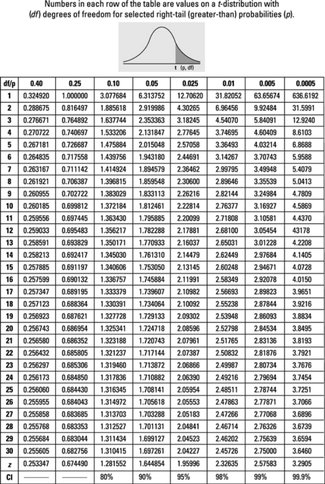
The sample size is made up of 1,000 observations. Suppose you want to test the null hypothesis that the slope parameter is equal to 0 against a 2-sided alternative at the 10% significance level. What is the relevant critical value of the test statistic? The t-table is at the end of the assignment paper.

Exercise 2

You estimate a regression of the form given by the equation below in order to evaluate the effect of various firm-specific factors on the firm’s return series. You run a cross-sectional regression with 300 firms:

Ri,t  = β 1 + β2 Sizei,t + β3 MBi,t + β4 Divi,t + β5 Betai,t + ui,t

where Ri,t  is the percentage annual return for the stock and

• Size is the size of firm i measured in terms of sales revenue

• MB is the market to book ratio of the firm

• Div is the dividend paid by the firm (in cash)

• Beta is the stock’s CAPM beta coefficient

You obtain the following results (with standard errors in parentheses):

Table 1: Regression Results

Notes: Standard errors in parentheses.

1. Calculate the t-ratios.

2. What do you conclude about the effect of each variable on the returns of a security?

3. On the basis of your results what variables would you consider deleting from the regression?

4. If the stock’s beta increased from 1 to 1.4, what would be the effect on the stock’s return?

5. Finally, explain why it is desirable to remove insignificant variables from a regression?

Exercise 3

The following model to forecast the stock market variance over the next period has been estimated. Using a sample of 1,000 observations, we want to test the accuracy of this forecast:

RVt+1  = −0.021 + 0.432IVt

where the stock implied variance IVt  is our proxy for the market realized variance forecast over the next period. The t-ratio associated with the intercept is -0.276 and that of the slope is 4.310.

• Based on the t-ratios, what can you say about the significance of these parameters?

• What is the standard error associated with each of these parameters?

• What is the 95% confidence interval associated with each of these parameters?

• Using the findings above, separately test the null hypothesis that the slope is equal to i) 1 and ii) 3.

Exercise 4

You are the commodity risk analyst in an investment fund. You are required to build a potential model in order to predict the next period(s) oil prices.  By using i) economic rationale and ii) academic literature, provide the following:

• Regression equation model

• Justification for the variables selected (please use academic literature references to support this point)

• Expected relationship and coefficients’signs between the dependent variable and the selected predictors.