Macro-Econometrics Homework Assignment #6
Hello, dear friend, you can consult us at any time if you have any questions, add WeChat: daixieit
Macro-Econometrics
Homework Assignment #6 (150 points)
The Excel file called HW_Data_Period_6.xlsx contains the logged real exchange rates for the U.S. relative to Canada, Japan, Germany (before the euro), and the U.K. The four series in the file are labeled RCAN, RJAP, RGER, and RUK, respectively. They are described further in Ender’s book. All series run from February 1973 to December 1989, and each is indexed so that the February 1973 value is equal to 1.00.
(a). Graph the level of RJAP – does it look stationary? Why or why not? Take the first-difference of this variable – call it DRJAP – does it look stationary?
(b). For RCAN, compute the ACF and PACF for the following three situations: (i) the real exchange rate in log levels, (ii) the first-difference of the levels, and (iii) the residuals from a regression of the level on a constant and a time trend. What do you conclude from the results as they relate to the stationarity of RCAN? Please be sure to discuss all three sets of results.
(c) Explain why it is not possible to determine whether a variable is stationary or non-stationary by simply looking at the ACF and PACF.
(d). For each of the real exchange rates, run the following ADF regression:
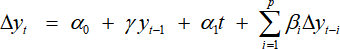
Set the number of lags (p) equal to 12, and report the t-statistics for γ in each of the four regressions. Why is it incorrect to use the usual normal distribution to evaluate whether γ is not statistically different from 0? What is the appropriate distribution to use in the particular case? What is the appropriate critical value? Using a significance level of 0.05, can you reject the null hypothesis that γ is not statistically different from 0? What does this mean for the stationarity of the data series?
(e). Impose the assumption that γ is indeed equal to 0. The next step is to test the relevance of the time trend. For each of the real exchange rates, run the following regression:
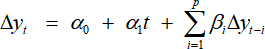
Set the number of lags (p) equal to 12, and report the t-statistics for the coefficient on the time trend. What is the appropriate distribution and critical value for testing whether the coefficient on the time trend is not statistically different from zero at the 0.05 level? What do you conclude?
(f). Now, assuming that there is no time trend, run the following ADF regression:
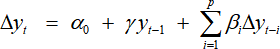
Again set the number of lags (p) equal to 12, and report the t-statistics for γ in each of the four regressions. What is the appropriate distribution and critical value to use in this particular case? Using a significance level of 0.05, can you reject the null hypothesis that γ is not statistically different from 0?
(g). Impose the assumption that γ is indeed equal to 0. The next step is to test the relevance of the constant. For each of the real exchange rates, run the following regression:
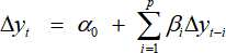
Set the number of lags (p) equal to 12, and report the t-statistics for the constant in each of the four regressions. What is the appropriate distribution and critical value for testing whether the constant is not statistically different from zero at the 0.05 level? What do you conclude? Does this make sense, given what you saw in part (a)?
(h). The final step is to test whether there is a unit root without including a constant or a time trend. What do you conclude?
(i) After all of these tests what do you conclude about the statistical behavior of the real exchange rate variables in log levels? Does this fit with our economic theories that describe the behavior of real exchange rates?
2023-07-10