Hello, dear friend, you can consult us at any time if you have any questions, add WeChat: daixieit

BIOL 5300 IDCGV 2022/23  Module 3 Computer Pract. Session 2.    GWAS analysis

In this exercise, you’ll get hands-on experience of running part of a GWAS association analysis - you’ll be given data for two individual chromosomes for two separate phenotypes and will run the analysis yourselves on those data using PLINK. The aim is to see how the analysis works by running commands/scripts that ask the question ‘are there any loci on this chromosome that harbour variation that predisposes to disorder A or to trait B?’ (or whatever we are calling them). You will also get the chance to practice your data cleaning and QC skills.

Each of you will be provided with the same two sets of files: one contains data for a dichotomous phenotype (e.g. Major Depressive Disorder, MDD) from a study using a case/control approach; the other contains quantitative trait values (e.g. IgE levels in blood) from a study investigating a continuously distributed trait.

Step 1 Get set up at the High Performance Cluster (HPC):

· start a vpn session running - this will be needed for all work at the HPC

· open a terminal session at HPC and log in - this is slightly different depending on whether you are using a PC or a Mac.

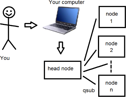
Details about how to open this session are below, but first here’s a diagram and description (courtesy of Joey Ward) that explains how things are organised up at HPC and how you get things to run on the nodes that make up the cluster:

When you log in to the HPC, you log into the head node. The head node isn’t very powerful and is really just there for you to make text files and submit jobs to the nodes. To send a job to a node you use the qsub command (think: submit to queue). Usually the thing you submit to the queue is a shell script which contains the commands you want to run (there’s more explanation about shell scripts below...)

To open your terminal session at HPC:

· if you are using a PC, use PuTTY or MobaXterm or a similar client

· the port is 22; the server address is:

headnode03.cent.gla.ac.uk

· Login: your username is your GUID i.e. 3434343t, including the letter at the end

· Password: you were given a temporary password for HPC during the Computing Bootcamp, and you should have changed it - if you didn’t, consult Mark or Joey*

· if you are using a Mac, use ‘Terminal’ and the ssh command; type:

ssh yourusername@headnode03.cent.gla.ac.uk

· Login: your username is your GUID i.e. 3434343t, including the letter at the end

· Password: you were given a temporary password for HPC during the Computing Bootcamp, and you should have changed it - if you didn’t, consult Mark or Joey*

· if the ssh command above does not work (e.g. if you get an error message), then there are three other things you can try - we suggest you try them in the following order:

· use the following command instead, which alters a ‘config’ file that sits in your user directory in your Mac:

ssh -o KexAlgorithms=+diffie-hellman-group14-sha1 -o
HostKeyAlgorithms=+ssh-rsa -c aes256-cbc
yourusername@headnode03.cent.gla.ac.uk

· create or modify a ‘config’ file inside a folder called ‘.ssh’ that is in your home directory on your Mac so that it contains the above information; its contents should look something like the following:

Host hpc

HostName headnode03.cent.gla.ac.uk

User yourusername

KexAlgorithms +diffie-hellman-group1-sha1

Ciphers +aes256-cbc

· try using a different terminal emulator, such as iTerm2 (available via the Apple App Store), or Termius (available via https://termius.com/mac-os)

· *to remind you - the first time you log in to HPC, you MUST change your password (if you’ve already changed your password in Semester 1, no need to do it again) - if you do need to do this, use the ‘passwd’ command at the command line prompt; your new password must conform to some ‘good password’ criteria e.g. it must not be simply a word that appears in a dictionary.

·  Note that you are asked to retype the NEW password - see the screenshot below (the prompt will be different at HPC):

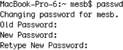
·  - don’t forget to do this or it will exit with an authentication error of some kind.

See hints and tips below (at the end of this document) about how to get PuTTY to behave properly in terms of colours of text and terminal window background

· your home directory at the HPC has the address:
/export/home/biostuds/<username>

· Please now get to know the contents of your filespace at the HPC ....:

· use your existing command line and filesystem computing skills learned during bootcamp (or elsewhere)

· e.g. look at the current directory structure using ‘ls’; or at all files and directories under the current directory using ‘ls -al’. Change directory using ‘cd’. Create new directories using ‘mkdir’ etc.

· consult websites that explain how Unix works and how a Unix filesystem is organised and interrogated

· see the ‘Hints and Tips’ Appendix at the end of this document...

Step 2

Obtain a functioning version of the program PLINK2; Joey Ward has kindly let us make copies of a version that he keeps in his filespace at HPC - type the following at the prompt after logging in to HPC*:
[for clarity, in the command below ‘·’ is a space character; ‘.’is a full stop character]

cp·-a·/export/home2/jw269k/plink/·.

*you can do this from your home directory:
/export/home/biostuds/<username>/
or you can create a subdirectory one level down from your home directory and ‘cd’ to that directory first before copying PLINK over.
Also, you’ll need to make sure that you have no other versions of PLINK already installed at HPC

· Your home directory (or whatever directory you copied the files over to) should now have several files (you copied these over together, the result of using the ‘-a’ flag in the cp command just now).
One of these files is the executable, plink; other files are either needed by PLINK or are for demo purposes (just ignore the latter).
There may also be a subdirectory also called ‘plink’, but probably not - if there is, just ignore it for now.

· List the files and directories inside the directory you copied PLINK over to by using the ‘ls -al’ command. Check you understand what files you copied over, which
one is the executable, and whether any subdirectories have also appeared.

· You can organise this bit of your filesystem however you like, you can make a new subdirectory underneath and move the executable into it if you want to, or not, as you choose - create a filesystem with a sensible structure that works for you. In the steps below you are going to add datafiles and then generate analysis output files - having these all in the same subdirectory can get confusing

· Do NOT create several levels of subdirectory all called plink - use different names for each level of subdirectory, or it will get even more confusing...

Step 3 you should now have plink in your home directory (or a subdirectory) - you need to add the location of the plink executable to your PATH so you can call it from any directory just using the command:

plink

...and not have to type the full path to the program i.e.:

/export/home/biostuds/<username>/plink_files/plink

· To do this you need to add information about the PATH to your existing .bash_profile file up at HPC. This file lives in your home directory and is read by the operating system (Unix) every time you log in to the HPC (you can force the OS to read it again while you are logged in as well, if you make any changes to it).

· From your home directory open the file .bash_profile using an editor* - nano or vi - and you will see the following:

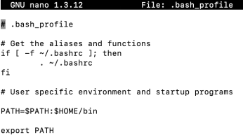
· Edit this file to add paths to the PATH line which already contains ‘$HOME/bin’ (or it may say ‘usr/bin’) Just add a colon (:) after $HOME/bin, then add the full path to the DIRECTORY that the PLINK executable is in i.e.:

/export/home/biostuds/<username>/plink_files

NOT

/export/home/biostuds/<username>/plink_files/plink

· Make sure you’ve added to your .bash_profile file at the HPC the path to ALL subdirectories you might need at HPC (i.e. all those holding program executables)

· Go back and do this step again every time you install a new executable file in your filesystem and/or move an executable to a different or new directory

· Remember always to use the full path to the directory containing the executable in the PATH command

· Once you have added the full path to the DIRECTORY that the PLINK executable is in, save the file and exit the text editor you are using

· You should now be back at your command line prompt. Type

bash <return>

· This forces the system to re-read and implement the commands in your .bash_profile file

*There is another way to edit the .bash_profile file - start a vpn session, transfer the .bash_profile file by ftp to your laptop/vPC, edit it in a simple text editor, then transfer it back up to the HPC; if you do it this way, you’ll need to remember to save it in text format, then remove the ‘.txt’ extension, and you’ll need to make sure that you save it with UNIX end of line (E.O.L.) characters; you may also need to alter the filename while it’s on your PC - don’t forget to change its name back to .bash_profile at the HPC

Please note - as we explain below, you must NEVER run PLINK with large datasets by calling it directly from the command line at your prompt at the HPC headnode - you will crash the system for everyone at Univ. of Glasgow...

See Step 7 below for how to run PLINK

Step 4 Alternative ways to get PLINK - only do this step if you find you need to after
Step 7; for now, skip straight on to Step 5....

If you cannot get PLINK to run properly in Step 7 below, try testing PLINK by running it with no input data from an interactive node session - see the section called ‘Testing your installation of PLINK to make sure it works’ below.

Here are some other ways to get PLINK and make it run:

· If the copy of PLINK that you have installed in your filespace at HPC is not working, then there are a few ways to obtain a copy that might work instead.

· option 1: Download the latest stable version of PLINK2 for the 64-bit Linux platform from https://www.cog-genomics.org/plink/1.9/ and upload it to your HPC account using WinSCP or FileZilla:

version 1.90 beta - build: stable (beta 6.21) Linux 64-bit: plink_linux_x86_64_20201019.zip

· Download this .zip file to your virtual PC (or your own computer) - you should NOT unzip the file at this point

· Rename the zip file to simply ‘plink.zip’

· Use FTP to move the .zip file to your HPC home directory (WinSCP, FileZilla etc.) - you’ll need to connect to the same HPC server address as above

· Make sure that you specify Port ‘22’ for the FTP connection in the dialogue box

· Unzip the .zip file - the command to do this will be something like:

unzip file.zip

· Note that if you are using a Mac, the file will be automatically unzipped when you transfer it to your home directory

· If the latest version of PLINK from the PLINK2 website does not run for you without error messages (something about ‘kernel too old...’ or similar), it may be that all our HPC nodes are running operating systems that are not compatible - you then have two other options, as follows:

· option 2: try a slightly older stable build from the PLINK 1.9 website (e.g. v.1.7)

· if you do this option, make sure you have deleted all other versions of PLINK from your HPC home space first

· option 3: add the path to Joey Ward’s copy of PLINK to your .bash_profile and call that copy when you want to run PLINK; add to your PATH:

/export/home/jw269k/plink/

· Be sure to remove the original path and save the updated .bash_profile. Then close down your terminal session at HPC (and quit PuTTY or whatever you have used to connect), then start it up again and sign back in to HPC again using your username and password. Now you are using Joey’s version of PLINK, which should work.

· If you are stuck on this bit, consult Joey or the demonstrators and we’ll give you a solution or workaround.

Step 5 Get to know PLINK - there are five ways to do this:

· use the instruction/command set on the left hand panel at the OLD PLINK homepage (http://zzz.bwh.harvard.edu/plink/) - look at the functions down to ‘Section 11. Association’

· use the instruction/command set on the left hand panel at the NEW PLINK homepage (https://www.cog-genomics.org/plink/1.9) - this may be quite hard to follow for novices

· go to the PLINK tutorial page (http://zzz.bwh.harvard.edu/plink/tutorial.shtml) linked from the old homepage and work through it. Using the example files (packed into ‘hapmap1.zip’) provided there may not work, but you can still follow the procedures they are describing to get a feel for how the analysis would proceed; alternatively you could try doing the tutorial, but using the exercise files you have been given by us (see below)

· listen to Joey Ward explaining what to do, and write it down....

· You could also try the GUI version - GPLINK - obtainable as a .jar file from http://zzz.bwh.harvard.edu/plink/gplink.shtml

The basic rule is that getting PLINK to do what you want it to do involves calling it from
the command line (CAVEAT - see Step 7 instructions below - YOU MUST NEVER RUN
THIS COMMAND FROM THE COMMAND LINE WHILE LOGGED IN TO THE
HEADNODE AT HPC), and adding ‘flags’, defined by ‘--’, all on one line, that give
instructions, e.g.:

plink --bfile /path/to/binaryformatdatafile --do-command
--command-option <option> --out /path/to/output/file

· Note: Never make the output file name the same as the input file name !!

· see the end of this exercise for some handy tips about PLINK commands and about using shortcuts in path definitions - (this list is NOT comprehensive, so you must also look at sources listed above for lots more commands and what they do)

Step 6 Obtain and prepare the data for the exercise

NOTE: Do not store datafiles in your plink directory (i.e. do not place them inside the directory that contains the plink executable).

You should place the datafiles in one of two places:

· Your home directory

     OR

· A new directory that you have created (using mkdir) for your data

It is also advisable to create a results directory containing at least two subdirectories called something like exercise_data and assessment_data. Doing it this way means all your software, data and results are neatly stored on the system making it easier to manage. Draw yourself a diagram of your directory structure to refer to so you don’t get lost...!

Obtaining the data for the GWAS exercise - Joey Ward has set it up and it can be copied from one of his directories at HPC; while logged into a terminal session at HPC, type:

cp /export/home/jw269k/biostuds/1234567.tar.gz .

This will copy the data to your current directory (as defined by that last ‘.’ in the command).

Unzip and unpack the .tar.gz file using the following combined command (make sure your .bash_profile file has the path to the /bin directory, where these unix command programs are stored):

tar -xzf 1234567.tar.gz

The dataset for the GWAS exercise consists of a set of datafiles - 12 files in all. These will have been extracted by the ‘tar’ command into a subdirectory called ‘1234567’

Inside the ‘1234567’ subdirectory, there are two further subdirectories, each containing data for ONE of the TWO different types of phenotype you’ll be analysing:

· ‘dichotomous’

· ‘quantitative’

For each of these phenotypes, there are data for each of TWO chromosomes

For each chromosome for each phenotype, there are THREE files

Thus, there will be 12 files in total - 6 files per subdirectory x 2 subdirectories:

    ‘dichotomous’ phenotype (‘dichotomous’ folder) - these are the 3 datafiles for chromosome 1 (there will be another set similarly named for chromosome 2...)

1234567_1.bed
1234567_1.bimF
1234567_1.fam

    ‘quantitative’ phenotype (‘quantitative’ folder) - these are the 3 datafiles for chromosome 1

1234567_1.bed
1234567_1.bim
1234567_1.fam

Some info to get you started:

· The datafiles are already in binary (machine code) format (.bed = ‘binary ped file; .bim = binary marker file etc.) - we could have provided them in a more ‘raw’ format as *.ped and *.map files but this format generates extremely large files, so they are not so useful when disc space is limiting (and the programme would probably have needed to convert them to binary format, adding time to the analysis).

· *.ped and *.map files have a format that is standard in the genetic analysis field (they used to be used in genetic linkage analysis). This format is still useful in certain circumstances. You may find that you do in fact want to create these .ped and .map files as output from your analysis, as they may be of use as input to other downstream analyses (see below) - there are PLINK commands to do this;
PLEASE NOTE - these are huge files - don’t do it unless you need to, make sure you have filespace available, don’t do it at the HPC (use your virtual PC) and don’t do it for whole chromosomes - only do it for a subset of markers.

· The size of the chromosomes in the dataset for this exercise is between 150Mb and 500Mb.

· The case/control study dataset has a few thousand cases and several thousand controls - find out how many there are of each using appropriate PLINK flags.

· The quantitative trait has both positive and negative values (you’ll hopefully be able to look at the distribution of this variable as part of the analysis you run).

· The genotypes have all been coded in the genotype file as ‘0,1,2’ so you can model SNP effects any way you like (e.g. ‘additive allelic effects’, dominant etc.) in the models you run.

· Phenotype has been coded as follows for the dichotomous disorder:

1 = unaffected

2 = affected

· PLINK reads ‘-9’ as missing data.

To check that your datafiles are actually in binary format, look inside the files (‘head’ and ‘less’ commands let you look, with or without scrolling)

head <filename>

less <filename>

· tip - to exit from these unix command programs, type ‘q’

 - you’ll see that for two of the three files, the contents are unreadable gobbledegook:

For the files you can read, note the contents - can you ascertain any of the following?:
column order, any missingness identifiers, order of alleles at each marker (e.g. is a 1,2 heterozygote always coded as ‘1 2’ or can it be ‘2 1’?), the delimiter character used between fields/columns.

Step 7 Start two types of analysis using PLINK on the HPC - don’t set these all running at the same time, we don’t want to overload the server; please note the caveats below BEFORE you start:

- Disease Condition A Case/control analysis

- try doing a number of different analyses using different types of model

- use the flags --assoc and --model to implement the various models/tests, e.g.
  1 d.o.f. Chi-Sq test, Cochrane-Armitage trend test, test for dominant effects

- use the flag --logistic to run a logistic regression (modelling genotype as
  additive allelic effects, 1 d.o.f.); this also allows you to add covariates, if
  any are supplied e.g. sex

- Quantitative Trait B QTL analysis

- use the flag --linear - this instructs PLINK to run a linear regression, modelling
  genotype as additive allelic effects (0,1,2)

- PLINK won’t let you run an ANOVA model with genotype coded as a categorical
  variable, but other programs available on the web may do so - if you feel like it, try
  to find one that will and run it that way too - note the differences from the linear
  regression result

BEFORE running any association analyses.....

- you MUST NOT submit jobs of this size for processing at the HPC using the ‘headnode’
servers (i.e. NEVER type plink <RETURN> (with appropriate flags) at the command line
prompt) - these jobs will overload the system and crash it for other users. Instead,
you MUST submit jobs via the ‘qsub’ command, which gets them put into a queue system
for jobs. (This ensures that big jobs, despite being called from the headnode, are NOT
actually RUNNING ON the headnode).

Note - do NOT do Step 7 using qsub in an interactive node session if you have
used this approach to test your PLINK installation initially.

To run PLINK on actual data, first write a shell script using Notepad++, TextEdit or Word -
call it something like ‘my_shell_script.sh’ (see exemplar file on the Moodle) -
containing the following lines, making sure that it is saved in unix shell script format (with
‘.sh’ extension, not ‘.txt’) and also has Unix E.O.L. characters and NOT Windows line
endings):

#!/bin/sh

#PBS -l walltime=1:00:00

#PBS -l cput=1:00:00

#PBS -l nodes=1:centos6:ppn=1

#PBS -m abe

#PBS -q bioinf-stud

#PBS -M your@studentemailaddressgoeshere

Commands to call and run a programme go here e.g. plink --bfile....etc., so replace
this text in italics with your command line code (it should NOT be in italics…). Make
sure you do NOT comment out this command line code (i.e. do NOT include a ‘#’ at
the beginning of the line

Note: the lines that start ‘PBS’ should contain a ‘#’ character.

Further note: you can include multiple lines with commands, it will run each of
them.

More further notes: you need to check the instructions below, or consult a
demonstrator, or consult the PLINK webpage instructions when constructing this
shell script to find out how to format the names of the input files and output files
when writing the plink command line into the file....

This shell script file tells the HPC how much time and computing power to allocate to each
job. If a job goes over that time, it will be stopped, even if it has not completed - you may
need to experiment with the walltime and cput parameters; ask Joey and the
demonstrators for advice about values to try for these parameters, and DON’T make them
big just because you want to guarantee the run will finish - spend time working out the
minimum values required, you’ll soon get a feel for it.

The ppn parameter tells the HPC how many processors to use per node in the cluster.
Setting this to ‘1’ should be sufficient for most jobs. If any repeatedly get stopped before
completion, you are permitted to increase this number to ‘4’ for those jobs only - do NOT
use a number this big as default. Jobs are closely monitored by HPC staff - going over that
number may result in your HPC privileges being taken away....

The cput parameter tells the HPC to kill the PLINK job after a specified time running on
the processors it gets allocated to; you will almost certainly need to increase this time for
your assessment data, as big jobs can take longer than 1 hour to run.

Put this file in your home directory at the HPC. You will submit this file to the queue when
you want to run PLINK (or other big jobs).

Note: you can have multiple shell script files with different instructions in (recommended),
or you can keep editing a single shell script to create the commands for each new run you
wish to carry out (NOT recommended).
If you have multiple files, change the name for each shell script you create to something
meaningful e.g. exercise_data_quantitative.sh or
assessment_data_logistic.sh depending on what plink command(s) the script
contains. Do not call them ‘my_shell_script1.sh’, ‘my_shell_script2.sh’ etc.
- you’ll soon forget which script you used to do which run.

The command line code required to run PLINK from inside your shell script should look something like the following, adapted for the paths and filenames you want to use:

plink --bfile /path/to/quantitativeinputfile \

--linear \

--out /path/to/outfile

· ‘bfile’ tells PLINK to expect input files in binary format

· as usual, replace the paths/filenames in italics with the location and name of the file you want to use, and don’t use italics!

· you do NOT need to include the extension (‘.bim’ etc.) from the inputfilename, nor include an extension for the output filename

· as stated above, never call the outfile the same name as the input file

· there are flags --fam and --bim if your fam or bim files start with filenames different to the .bed file, but we aren't going to do that

· the ‘\’ character tells PLINK that the next flag is part of the same command i.e. it avoids the problems caused by having a line return or end of line character part-way through the command - it’s therefore OK if your command runs over multiple lines in your shell script

·  you can use the shortcut to your home directory (see hints and tips below) instead of the full path if you want - deploy the ‘~’ Tilde character correctly

Then set the job running via qsub by typing at the command line prompt:

qsub my_shell_script.sh

Once your job has been submitted successfully, check its status whenever you want using the qstat command, with flags:

qstat -a -u username

In the status (‘s’) column, you can see the status of the job

Q = still queued, not yet running

R = running

C = complete (may indicate stopped/crashed out with an error, rather than finished)

Once the job is complete, go and find your output files (look in the correct directory, as specified in the run command in your shell script!).

· Tip - a logfile and an error file are generated in every run - if the error file is empty, and the Exit code in the log file = 0, then everything ran OK.....!

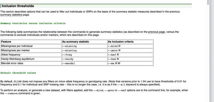
Run the analysis again using a slightly more sophisticated set of parameter settings involving some QC and/or filtering within your shell script e.g.:

plink --bfile path/to/quantitativeinputfile \
--linear \
--maf 0.01 \
--hwe 1e-6 \
--out /path/to/outfile

Think about what these extra flags do and why we might want to use them...
Your job here is to work out the optimal set of QC and filtering flags for the analysis you are doing.

Step 8 Review the results summary information provided by PLINK and make sure you understand which the important columns are and what they mean

Note:

· PLINK’s output files report the effect size/direction for the minor allele (even though genotype is recorded as ‘0,1,2’ for the major allele in the input file... - go figure...)

· The ‘A1’ column - make sure you read the PLINK helpfiles so you understand which allele is designated as allele 1 - it could be the first allele in the raw data file, or the first allele alphabetically, or the minor allele, or the reference allele, or the non-reference allele; and make sure you know whether the OR and Beta column reports results for the same allele as in the ‘A1’ column or for another allele

· The NMiss column tells you how many indivs. were INCLUDED in your analysis (which relates to your power) - it stands for ‘Non-Missing’

Step 9 Run various types of QC on the data and ascertain the effect of these on the results of your association analysis

· find out whether any indivs have >5% missing marker genotype data; if yes, exclude them

· find out whether any markers have missing data for >1% of samples (indivs); if yes, exclude them

· try filtering out markers that fail the HWE test at some specified level (don’t make this too stringent...)

· for each of these, you can run the query/test in PLINK, or you can try doing it in R

Step 10 Use R to plot a Q-Q plot and a Manhattan plot; use Haploview also

Use the base R package to plot a Manhattan plot, roughly (replace the filename ‘plinkoutputfile.linear’ with the actual filename of your output file(s); replace the variable names with the real variables/column titles in those files):

#read table into R

chrom <- read.table("plinkoutputfile.linear" , header = T)

#make manhattan plot

plot(chrom$BP, -log10(chrom$P)

#make a table containing only e.g. genome wide signif. hits

sig_results <- chrom[which(chrom$P <= 5e-8),]

You should also be able to plot a nicer Manhattan plot - there are three ways to do this:

· Add plot detail to the R plot function above.

· Use the R package ‘qqman’ to make both QQ plot and Manhattan plot. You’ll need to download it from CRAN (https://cran.r-project.org/web/packages/) and install it first.

· The two useful functions in the ‘qqman’ package are manhattan() and qq().

· Work out what file format ‘qqman’ uses as input - either make PLINK give you output in that format or create a file (containing chromosome, position, marker ID and p-value data - make sure some of the p-values are pretty small...).

· The manhattan() function takes a data frame that contains chromosome number, base position and p-value. It is designed to work with the output files of PLINK.

· The qq() function only needs a list of p-values. Example calls of these functions would be:

manhattan(my_plink_summary_stats)

qq(my_plink_summary_stats$P)

· NOTE - we have also given you a ‘real’ PLINK output file (from a real analysis that Joey did using UK Biobank data) to plot a Manhattan plot for, so you can see what they really come out like (see Moodle Module 3: the file to use is ‘mdd_hits.assoc’).

· Use the Haploview package.

· Download and install Haploview on your vPC (or your own laptop) - go to https://www.broadinstitute.org/haploview/downloads, download the jar file (do not use the .exe installer file, it won’t behave properly). If the jar file is compressed, uncompress it using 7-Zip or WinRAR, or whatever compression software you have on the virtual PC or your own computer.

· Run Haploview by double clicking on the jar file, or from a terminal session by calling it:

prompt$ java -jar Haploview.jar

· Use the tutorial (https://www.broadinstitute.org/haploview/tutorial) and example files available on the download webpage to explore what Haploview does.

· To plot a Manhattan plot, Haploview will need as input two files you already have by this point:

· the PLINK analysis output file

· the *.bim marker info file

· Select ‘Open new data’ from the menu, select the ‘PLINK FORMAT’ tab, and select these two files as input files in the dialogue box. Use the menu options (see the ‘Plot’ pop-up button in the dialogue box) to create the Manhattan plot - you should be able to set the plotting parameters to achieve an attractive and fully informative plot.

OTHER THINGS TO TRY:

Step 11 We’d like to be able to use LocusZoom to inspect an association analysis hit.
Go to http://locuszoom.sph.umich.edu/locuszoom/

It is possible to plot your own analysis output data at LocusZoom, but because your exercise (and assessment) data are simulated, the SNP IDs, though real, do not correspond to their real chromosomal coordinates (which Locus Zoom will look up from online DBs), so it will probably fail or give you a meaningless plot.

As an alternative, to show you how it works, we have provided you with some demo output files either from our own GWAS, or from colleagues or from the community at large (see ‘mdd_hits.assoc’ and ‘BMI-Metaanal_Locke_UKBiobank_2018.xlsx’ files in Module 3 on the Moodle). Try plotting the region around any of the GW-significant hits in either dataset.

You need to run LocusZoom using the ‘Legacy Services’ section of the webpage:

· choose a published dataset and look at its results using the ‘Interactive Plot’ tool

· upload either of the files above using the ‘Single Plot’ tool; if you use the ‘mdd_hits.assoc’ file for this, you’ll need to check the column titles in this file and make sure they match what LocusZoom expects; please also note that this file has space-separated data - to get this to open in LocusZoom you’ll have to convert it to a tab-separated format - do this by opening in either R or Microsoft Excel and saving/exporting it in the required format.

Step 12 Calculate how much power you had in this GWAS exercise to detect association under different parameter settings - go to the GAS association study power calculator at http://csg.sph.umich.edu/abecasis/gas_power_calculator/index.html

Use the sliders to set your input parameters - no. of cases and controls, alpha value for significance etc. Use the default (‘multiplicative’) disease model; set the prevalence, disease allele frequency and genotype relative risk (akin to odds ratio) to a range of different values. Look at the output - ‘power’ is the probability that you will get at least one significant ‘hit’.

Also find out how many cases and controls you would need for 80% power (i.e. to get a significant hit 8/10 times you run the analysis).

Step 13 Look at the LD structure of the region around any GW significant association hits you have uncovered in the two exercise datasets

Use Haploview to look at LD in a subset of your markers.

· take several random markers and work out whether any are in LD with each other

· are any markers that are close to any significant lead SNPs you’ve found in the exercise in LD with the lead SNP, or with each other?

To generate an LD heatmap, Haploview requires the individual-level genetic data. These are not present in your association analysis output file and Haploview cannot read the .bed input datafile. You therefore need to produce the ‘raw’ datafiles (*.ped and *.map).  PLINK can do this for you - use the --recode flag. Only do this for a smallish subset of markers, NOT the whole chromosome, and do it at the HPC but delete the files after copying them to your computer/vPC (see advice further up, and in the hints and tips section below).

You then have to edit the files before using them as input to Haploview

· the *.ped file must have missing data in the ‘phenotype’ column (for affected status or quantitative phenotype value) coded as 0, not -9

· for quantitative data, you must also replace all the data in the phenotype column with ‘0’

· the *.map file should contain only two columns - the marker rsID and the chromosomal coordinate as position in bp. (As LD is only calculated between SNPs on the same chromosome, the chr column is not relevant).

Import the *.ped and *.map files into Haploview using the dialogue box on the ‘Linkage format’ tab, then navigate to the LD calculation and plotting options in the menu system.

You may not be able to get Haploview to do what you want here - or it may take too long and you may have to kill the process! So....

You should also try calculating and plotting LD for some of the markers from your dataset in R

· do NOT use the whole chromosome!! It will never finish...)

Step 14 How to obtain the data for your GWAS task for the assessment:

Joey Ward has prepared the data and made it available to you.

It can be copied from one of his directories at HPC; while logged into a terminal session at HPC, type:

cp /export/home/jw269k/biostuds/yourstudentID.tar.gz .

This will copy the data to your current directory (as defined by that last ‘.’ in the command).

Appendices

Testing your installation of PLINK to make sure it works

If you are having trouble getting PLINK to run at the HPC using a shell script, there is a way to test whether the program itself is installed properly and working, by running it directly from a node using an interactive session.

· At the start of this document we said that usually you submit jobs (shell scripts with commands) to the HPC nodes to run the jobs as the headnode isn’t powerful enough to run multiple jobs simultaneously. Instead of submitting a job to a node, there is also a way to log onto a node directly so we can type commands on the node. To do this we also use qsub but with -I flag to make it an Interactive session:

qsub -I -l nodes=1:centos6:ppn=1,walltime=24:00:00

Below is a breakdown of what each term does in this command

· qsub

o a unix program executable that tells the OS to submit a job to the queue

· -I

o This is a capitol I (for India); it creates an Interactive session so you can log onto a node and enter commands directly.

· -l

o This is lower case l (for lemon) and is a flag that tells qsub that a list of job parameters and settings will follow

· nodes=1

o job requires one node (see diagram in Step 1). Larger jobs may require more nodes.

· centos6

o directs the queuing system to ensure that the job is sent to a node that has the operating system ‘Centos version 6’

· ppn =1

o each node contains several processors. If your job requires parallel processing you can request more processors.

· walltime=24:00:00

o this request means that the interactive session will last for 24 hours which is more than enough time to type “plink” and see what happens!!! 

If you look at the shell script in Step 7 (and the example script on Moodle), you will
see these settings and parameters in the top few lines after the ‘#PBS’ comment -
these are not in fact ‘commented out’ - the OS knows it needs to pay attention to
these, in this case.

Look at the other settings and parameters in the shell script (extra ones that are not in
the command for the interactive session above) and make sure you know what they
are doing.....

· After a minute or so you will be back on the command line - to start up PLINK just type:

plink

· If the previous installation steps have been successful and if the version of PLINK you have downloaded is actually runnable, then you will get a message about all the different flags you can use with PLINK. To get back out of the interactive session and back to the headnode type:

exit

· If instead of the above you get an error about how the plink command isn’t found, first exit the interactive qsub session using:

exit

· Then double check that the path you added to your .bash_profile is spelled correctly and the PLINK executable is in the correct location in your home directory. Close down PuTTY or terminal and then open them again and log back into the headnode. Then do an interactive session using the qsub command (with flags) above and try running plink again.

HINTS AND TIPS

- genotype gets coded as ‘0,1,2’ in the derived genotype/phenotype file made by PLINK after you run it. In the input file, this is equivalent to ‘no. of copies of the major allele’; however, in the output files, the result is given in terms of A1, which is always given as the minor allele - i.e. if you are running a regression model, a positive beta in the output implies that the minor allele is the risk allele. If you want to run a model under an assumption of fully dominant effects, there is a PLINK flag for this that should work with this coding system.

- you cannot run big PLINK jobs, such as a whole chromosome’s-worth of data in a GWAS, from the headnode at the HPC. You MUST use the job queuing system (qsub), otherwise you’ll crash the system for all the other users and it will take some hours to sort out!

- some useful PLINK flags to check out:

specifying format of input files:

--bfile tells plink you are supplying files in binary format already

--recode converts binary format files to ordinary format files .ped and .fam
the files get much bigger so ONLY do this at the HPC, only do it for
a SUBSET of markers* on one chromosome (before moving these
files to your virtual PC), and ALWAYS delete the new files after use

*selecting subregions of your data files to work with:

--chr

--from-bp (or from-mb etc.)

--to-bp

filters for QC:

--hwe

--maf

--mind

controlling the format and content of the output:

--out

--ci

--hide-covar

organising your input when running multiple models:

--script

- some useful Unix commands:

head <filename> shows you the first 10 lines/rows of a file

tail <filename> shows you the last few lines of a file

more <filename> scrolls through a file one screen’s worth at a time; use <ESC> to exit
from scrolling

less <filename> scrolls through a file one screen’s worth at a time, but you can scroll
backwards as well as forwards; use <ESC> to exit from scrolling

~/ indicates ‘home directory path’ - use this INSTEAD OF
/export/home/biostuds/yourusername, NOT in addition to this bit of
the path

chmod lets you change file permissions to make a file readable or executable
etc. For example, to make a program (such as PLINK) executable if it
isn’t already so, type at the command line prompt:

 chmod 777 pathtofile/filename

then look at the permissions (using ‘ls -al’) - you’ll see what the
setting ‘777’ does.

- Tips for FileZilla:

· When examining files to see whether the contents have been updated after a file transfer or editing process, make sure you refresh the contents of the window showing the directory listing - it doesn’t always update that listing on its own

· be careful when installing this program - some downloads are infected with malware...

- PuTTY - how to change the colour scheme:

Click on the ‘System’ menu at the upper left corner of the PuTTY window.

· Select Change Settings > Window > Colours.

· In the box that says "Select a colour to adjust", choose ANSI Blue and click the Modify Button.

· Slide the black arrow on the right up until you see a lighter shade of blue that you like.

· Click OK.

· Perform the same steps for ANSI Blue Bold so you can have a perceptible difference between the two.

· When you're finished, click Apply.

Additional note:

· the word ‘binary’ has two meanings for a computational geneticist! Please work out which one of these applies whenever you see the word used.....

· binary files - computer files written in machine code (rather than natural language), unreadable by humans unless you have an APP that can decode it

· a ‘binary’ phenotype -i.e. a dichotomous condition/trait, with ‘Cases’ and ‘Controls’ as the outcome variable in the word equation; or a predictor variable with two levels (e.g. ‘exposed’/’unexposed’, ‘male’/’female’ etc.)
- we are trying NOT to use the word ‘binary’ to indicate ‘dichotomous’ in or