1 Run the following code in R.

set.seed(2022)

sample(letters[1:8], 4, replace = FALSE)

Use the output from the above R code to select the keywords you need to answer from the list below. For example, suppose the result for the above code is “d”, “c”, “f” and “g”, then you should select keywords “d”,  “c”,  “f” and “g” from the list below to answer this question.

Note:  Please make sure to replace the seed used in the above R code with your student ID to select the keywords you need to answer this question.  We will not award the marks if you do not choose the keywords allocated to you based on your seed.

Write at least three informative sentences in the context of STATS 326/786 about the keywords selected from the list below. You shouldn’t copy the content available on the internet. Use your own words to explain the keywords.

Time series decomposition

•  This is a useful technique for understanding the nature of the time se- ries components, such as how trend-cycle and seasonal components have evolved over time. These features could assist us in building a forecasting model.

•  There are various ways of performing time series decomposition: classical decomposition, STL, X-13-ARIMA-SEATS.

•  Time series decomposition can also be used to forecast time series data by first forecasting the seasonally adjusted data and then adding back in the seasonal component of last year.

AIC and adjusted-R2  in regression

•  AIC and adjusted-R2  can be used to select the best predictors to use in a model.

•  Both AIC and adjusted-R2  penalize for model complexity; however, AIC is preferred over adjusted-R2   as the latter measure tends to select too many predictors.

•  Both of these measures cannot be used to determine whether the response variable needs a transformation or not.

Time series cross-validation

•  Time series cross-validation is a useful technique to determine the fore- casting ability of a model.

•  There are various methods of doing cross-validation:  rolling forecast ori- gin, rolling forecast window etc.

•  Time series cross-validation is generally preferred over simple training and test split as we get many out-of-sample comparisons if the time series is

long enough.

Box-Cox transformation

•  Box-Cox transformation is a mathematical transformation which includes both logarithm and power transformations.

•  If the data show a variation that increases or decreases with the level of the series, then a transformation can be useful.

•  When we use Box-Cox transformations for forecasting purposes, the back- transformed point forecasts will not give the mean of the forecast distribu- tion; they usually provide the forecast median if the forecast distribution on the transformed space is symmetric.

Correlogram

•  Correlogram is useful to visualise how the sample autocorrelations change with lags.

•  For time series with a strong trend, we observe that autocorrelations are large and positive and decay slowly as the lags increase.

•  For time series with strong seasonality, we can observe that autocorrela- tions multiples of the seasonal period are larger than other lags.

MAPE and MASE

• Both are scale-independent measures.

•  If the series are measured on different scales, we can’t use both measures to compare forecast accuracy across the series.

•  MAPE  is  not  defined  for  series with zeros,  and  MASE  is  more robust to this as the scaling factor comes from the MAE over the training set of a simple forecasting method such as naive for non-seasonal data and seasonal naive for seasonal data.

Forecasts from the random walk with a drift model

•  Random walk with a drift model: yt = 6 + yt−1 + et, where 6 is the drift term, et ∼ N(0, a2).

•  The model can be useful to forecast non-seasonal data with a linear trend: the forecasts from this model are similar to extrapolating the first and last observation into the future.

• The forecast distribution is ŷT+ℎ|T ∼ N (yT + ℎ gT(T)1(g)1 , â √ℎ(1 + ℎ/T)), where â 2 is an estimate of a2 and T is the length of the time series.

Prediction intervals

•  A prediction interval gives an interval within which we expect the future value to lie with a specified probability.

• If the distribution of the future observations is Gaussian we can construct 100(1 − a)% prediction interval as ŷT+ℎ|T ± Xa/2%â ℎ , where â ℎ is an esti- mate of the standard deviation of the ℎ-step-ahead forecast distribution and Xa/2% is the  100(1 − a/2)-th percentile from the standard normal distribution.

•  If the distribution of the future observations is not Gaussian and takes a complicated form, we can use bootstrapping to construct a prediction interval. [Total: 24 marks]

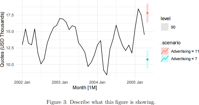
2 Figure 1 shows monthly quotes for a US insurance company from January 2002 to April 2005 in thousands of US dollars (40 months in total), and Figure 2 shows these monthly  quotes versus  monthly television  advertising  expenditure  from  January

2002 to April 2005 in thousands of US dollars.

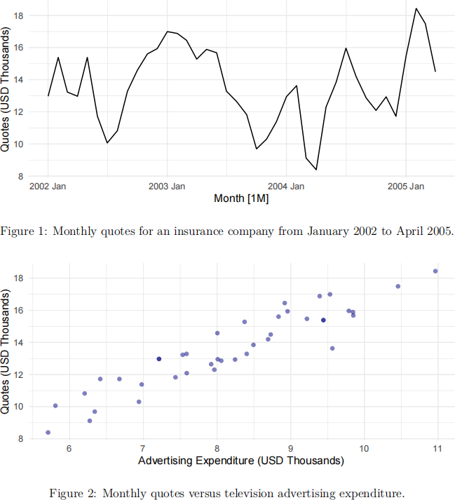
a Comment on the features you observe in Figures 1 and 2.                  [4 marks]

Solution:  Monthly quotes appear to have a flat trend in time,  and do not appear to have a seasonal pattern. Variability appears to be constant through time. Monthly quotes appear to have a strong positive linear association with monthly television advertising expenditure.

b Below is some R code for a time series regression model. Write the time series regression equation.         [3 marks]

fit <- data %>%

model(TSLM(Quotes ~ Advertising + trend()))

Solution:  Quotest  = p0 + p1 Advertisingt + p2t + et , where et  ∼ N(0, a2 ).       c Below is the R output of the fitted time series model.  Interpret the estimates

of the parameters of the two predictor variables.                                    [3 marks]

## Series: Quotes

## Model: TSLM

##

## Residuals:

##   Min     1Q Median    3Q   Max

## -2.215 -0.580  0.066  0.595  1.354

##

## Coefficients:

##            Estimate Std. Error t value Pr(> |t|)

## (Intercept)  -0.0314    0.7963   -0.04   0.9688

## Advertising   1.7635    0.0980   17.99   <2e-16 ***

## trend()     -0.0381    0.0110   -3.45   0.0014 **

## ---

## Signif. codes:

## 0 '*** ' 0.001 '** ' 0.01 '* ' 0.05 '. ' 0.1 ' ' 1

##

## Residual standard error: 0.789 on 37 degrees of freedom

## Multiple R-squared: 0.897,  Adjusted R-squared: 0.892

## F-statistic:  162 on 2 and 37 DF, p-value: <2e-16

vertising expenditure is associated with a $1.76 increase in quotes (or a $1000

ance quotes).  Holding advertising expenditure constant, p̂2  = −0.04 means

that for every month, we expect a $40 decrease in insurance quotes.

d Discuss  whether  you  believe  this  time  series  model  would  be  improved  by including seasonal factors as a predictor variable.   How would you test this belief?                 [5 marks]

Solution: Although the data is sub-annual (monthly), the plot does not appear to be seasonal, so we would not expect seasonal factors to improve the model. We could include season() as a predictor variable (with 11 dummy variables in  total)  into  the  time  series  model  and  compare  the  original  model  with the new one using information criteria such as AICc.  We would avoid using adjusted- 2  as this tends to over-fit.

e  (786 Only) If the season() function did not exist and you had to write your own seasonal dummy variables to include in the time series regression model, write the R code that would create the February and March dummy variables

for this monthly time series.

Solution:

data %>%

mutate(S2 = month(Month) == 2) %>%

mutate(S3 = month(Month) == 3)

f Assume that we have an ex-ante forecast of advertising expenditure for May 2005 of 9 (remembering that the units are thousands of USD). Using the fitted model, along with the additional R output below, compute a (one-step ahead) point forecast and 95% prediction interval for the insurance company’s quotes for May 2005.         [5 marks]

X <- cbind(rep(1, 40), data$Advertising, 1:40)

x.star <- c(1, 9, 41)

t(x.star) %*% ginv(t(X) %*% X) %*% x.star

##      [,1]

## [1,] 0.106

fit %>% glance() %>% pull(sigma2)

Solution:  Qutes41 = p̂0 + p̂1 × 41 + p̂2 × 9 = 14.31 and the 95% prediction

($12700, $15800).

u <- as.vector(t(x.star) %*% ginv(t(X) %*% X) %*% x.star) sigma2 <- fit %>% glance() %>% pull(sigma2)

beta <- fit %>% coefficients() %>% pull(estimate)

yhat <- sum(beta * c(0, 9, 41))

ci <- yhat + c(-1, 1) * qnorm(0.975) * sqrt(sigma2) * sqrt(1 + u) yhat

## [1] 14.3

ci

## [1] 12.7 15.9

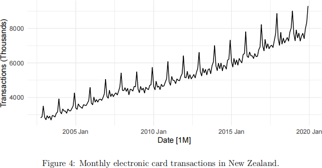
g Describe what  Figure 3 is showing and write the R code that was used to compute the forecasts.      [6 marks]

Note: Do not write the code to produce the plot.

Solution:  The figure shows some scenario-based forecasting.  The 90% predic- tion intervals and point forecasts for May 2005 (i.e., a one-step forecast) are computed under two different scenarios; when advertising expenditure is equal

to 7 and 11. For an advertising expenditure of 7 and 11, we get point forecasts of 11.6 and 18.4 quotes for May 2005, respectively.

future_scenarios <- scenarios(

`Advertising = 7` = new_data(data, 1) %>%

mutate(Advertising = 7),

`Advertising = 11` = new_data(data, 1) %>%

mutate(Advertising = 11))

fc <- forecast(fit, new_data = future_scenarios) [Total: 30 marks]

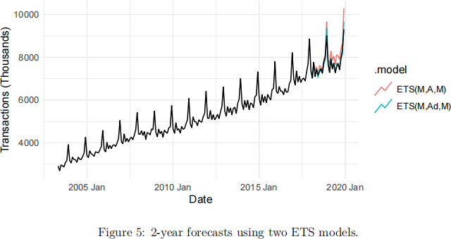
3 Figure 4 shows monthly electronic card transactions in New Zealand from October 2002 until December 2019. The tsibble object contains two variables: Date which gives the month, and Total which gives the total electronic card transaction count.

a Assuming the tsibble object is called data and the format for the date for the first observation is 2002 Oct, write the R code to create a training data set from October 2002 until December 2017.                           [4 marks]

Solution:

training <- data %>% filter(Date <= yearmonth("2017 Dec")).

b An ETS(M, A, M) and ETS(M, Ad, M) are fitted to the training data, and a 2-year forecast is displayed in Figure 5. Based on this figure discuss which ETS model is Model 1 and which is Model 2 in the following R output.    [3 marks]

## # A tibble: 2 x 4

##   .model   MAE MAPE MASE

##      

## 1 Model 1  296.  3.76 0.974

## 2 Model 2  109.  1.37 0.360

Solution: Model 1 is ETS(M, A, M) and Model 2 is ETS(M, Ad, M). From the figure, the ETS(M, Ad, M) forecasts are much closer to the true observations, meaning we would expect forecast accuracy measures such as MAE, MAPE, and MASE to be smaller.

c Interpret the estimates of  (a, p* , V, ) for the ETS(M, Ad,  M) model using

the R output below.                                                                                          [4 marks]

fit %>%

select(`ETS(M,Ad,M)`) %>%

report()

## Series: Total

## Model: ETS(M,Ad,M)

##   Smoothing parameters:

##    alpha = 0.314

##    beta  = 0.058

##    gamma = 1e-04

##    phi   = 0.975

##

##   Initial states:

##  l[0] b[0]  s[0] s[-1] s[-2] s[-3] s[-4] s[-5] s[-6] s[-7]

##  2740 40.1 0.949  0.97 0.983 0.934 0.987 0.967  1.03  0.95

##  s[-8] s[-9] s[-10] s[-11]

##  0.988  1.22   1.03      1

##

##  sigma^2: 2e-04

##

##  AIC AICc  BIC

## 2533 2537 2591

Solution:  。̂ = 0.314 which means the level changes slowly with time.  p̂∗ = 0.058/0.314 = 0.185 which means the slope changes slowly over time.  V̂  = 0.0001 which  means the  seasonality  hardly  changes  over time. ̂ =  0.975 which means there is a slow dampening effect.

d Discuss whether you believe an additive Holt-Winters model would be a bet-ter model for the electronic card transactions data set than the ETS models

already fitted in this question.                                                                      [3 marks]

Solution: The data exhibits multiplicative seasonality where the seasonal vari- ations are changing proportional to the level of the series. Therefore it makes more sense to use a multiplicative Holt-Winters model rather than an additive

one.

e Discuss  the  similarities  and  differences  between  the  additive  Holt-Winters model and the ETS(A, A, A) model.                            [7 marks]

Solution: The additive Holt-Winters model (sometimes called triple exponen- tial smoothing) is an exponential smoothing method with three smoothing equations;  one for the level,  one for the trend,  and one for seasonality.   It assumes additivity of error, trend, and seasonal components.  It can be used to produce point-forecasts when data is trending and exhibits additive season- ality.  It is a recursive algorithm and a non-linear optimisation routine.  The ETS(A, A, A) model is a state-space model that consists of a measurement equation that shows the relationship between our observed and unobserved (latent) states, and state equations that show the time evolution of our states (level, trend, seasonal).  It is a statistical model because we specify a proba- bility distribution for the innovation errors.  The ETS(A, A, A) state-space model produces the same point-forecasts as the additive Holt-Winters model, but can also produce prediction intervals to quantify uncertainty in forecasts. This is done by assuming an error distribution for the innovation errors, noting here that for the ETS(A, A, A) model, the innovation errors are the same as the regular residuals (additive errors). The ETS class of models are therefore more useful than exponential smoothing methods as we can get prediction bounds on our forecasts (and a forecast distribution). [Total: 21 marks]

4 For this question, consider the same monthly electronic card transactions data from Question 3.

a Discuss why you would  log transform the electronic  card transactions  data

before  fitting  an  ARIMA  model  to  this  time  series,  and  what  impact  this would have on prediction intervals of forecasts.                                      [3 marks]

Solution: We would log transform this data to stabilise the variance, making the patterns in residuals more constant over time.  We would have to back- transform the data to the original scale which will now make the prediction intervals non-symmetric around the point-forecasts.

b Describe how you would manually determine a candidate ARIMA model for this electronic card transactions time series.        [6 marks]

Solution:  As the data has a seasonal pattern, we would seasonally difference the data set first to see if we get a stationary time series.  If the data is still trending  after  seasonal  differencing,  we  would  difference  the  data  until  we remove the trend. This differencing will determine orders d and D. We would

then  look  at  the  ACF  and  PACF  of the  differenced  time  series .   We  would

expect a non-seasonal AR order p if the ACF exhibits exponential decay or sinusoidal behaviour and if the PACF has a significant spike at lag p and none beyond this.   Alternatively, we would expect a non-seasonal MA order q  if the PACF exhibits exponential decay or sinusoidal behaviour and if the ACF has a significant spike at lag q and none beyond this.  For the seasonal AR and MA orders, we would look at the seasonal lags in the ACF and PACF. For a monthly time series this lags with a multiple of 12. We would expect a seasonal AR order P if there is exponential decay in the seasonal lags of the ACF and spikes at the seasonal lags P (and none beyond this) in the PACF. Likewise, we would expect a seasonal MA order Q if there is a spike at seasonal lag Q in the ACF and none beyond this, as well as exponential decay in the seasonal lags of the PACF.

c Below is the R output from automatically fitting an ARIMA model to the log of the number of electronic card transactions.   The stepwise algorithm has been utilised. Write down the equation for this ARIMA model using backshift notation.              [4 marks]

fit <- training %>%

model(ARIMA(log(Total), stepwise = TRUE))

fc <- fit %>%

forecast(h = "2 years")

report(fit)

## Series: Total

## Model: ARIMA(3,1,0)(1,1,2)[12]

## Transformation: log(Total)

##

## Coefficients:

##          ar1     ar2    ar3     sar1    sma1    sma2

##      -0.7694  -0.3735  0.108  -0.0409  -0.482  -0.255

## s.e.   0.0766   0.0928  0.077   0.2580   0.247   0.165

##

## sigma^2 estimated as 0.000197:  log likelihood=484

## AIC=-955  AICc=-954  BIC=-933

Solution:

The selected model is: ARIMA(3, 1, 0)(1, 1, 2)12 .

The model can be written using the following backshift notation:

(1 − 1 B − 2 B2 − 3 B3 )(1 − Φ 1 B 12 )(1 − B)(1 − B 12 ) log yt

=   c + (1 + Θ 1 B 12 + Θ2 B24 )et ,

where et ∼ N(0, a2 ).

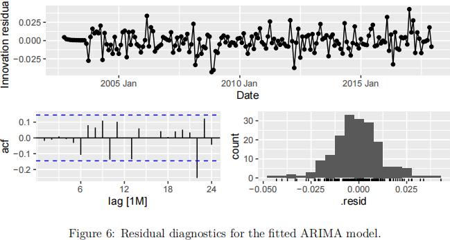
d Figure 6 displays the residual diagnostics for the fitted ARIMA model.  The R output for the Ljung-Box portmanteau test is also displayed below.  [6 marks]

## # A tibble: 1 x 2

##   lb_stat lb_pvalue

##        

## 1   35.6  0.00514

i Using the residual diagnostics from Figure 6, along with the R output to discuss the validity of the ARIMA model assumptions.                [4 marks]

Solution: Residuals appear normal with zero mean and constant variance over time. However, there is one significant lag at 22 in the ACF plot that suggests residual autocorrelation.  This has been tested with a portman- teau test, which rejects the null hypothesis that the residuals are indepen- dently distributed, indicating that there is indeed residual autocorrelation not captured in the model.

ii The Ljung-Box test for this question used ℎ = 24 lags.  What was the degrees-of-freedom value for this test?       [2 marks]

Solution: There are 7 model parameters estimated.

e  (326  Only)  Consider an AR(1) process with 1   =  −0.9.   Derive and write down the first three coefficients of the MA(∞) representation of this process. [6 marks]

Solution:  By sequentially substituting in the previous time period’s AR(1) equation, we end up with an MA(∞) representation that looks like:

t  = et + 1 et−1 + 1(2)et−2 + 1(3)et−3 + … ,

meaning the first three coefficients are ( 1 , 1(2), 1(3)) = (−0.9, 0.81, −0.729).      f (786 Only) Consider an AR(2) process with 1  = 0.9 and 2  = −0.9.  Derive

and write down the first two coefficients of the MA(∞) representation of this

process. You must show your working.                                                       [6 marks]

Solution:

t     = 1 t−1 + 2 t−2 + et

= 1 ( 1 t−2 + 2 t−3 + et−1 ) + 2 ( 1 t−3 + 2 t−4 + et−2 ) + et

…

=   et + 1 et−1 + ( 1(2) + 2 )et−2 + ( 1(3) + 2 1 2 )et−3 + …

( 1 , 1(2) + 2 ) = (0.9, −0.09).

cally equivalent to an ETS(A, N, N) model where a1  = a − 1.           [6 marks]

Solution: The ARIMA(0, 1, 1) model can be written as

The ETS(A, N, N) state-space model has the following measurement equation and state equation:

t     =   lt−1 + et

t − t−1 =   lt−1 + et − (lt−2 + et−1 )