STATS 786 STATISTICS SEMESTER 1, 2021
Hello, dear friend, you can consult us at any time if you have any questions, add WeChat: daixieit
STATS 786
SEMESTER 1, 2021
STATISTICS
Special Topic in Statistical Computing
(Time Series Forecasting for Data Science)
NOTE: For constants a and b , (a + b)2 = a2 + 2ab + b2 .
1 Select FOUR of the following scenarios. State whether the underlined statements are true or false. You MUST provide reasoning for your answer.
a Consider a time series generated from the following model:
yt = p0 + p1t2 + yt−12 + ![]() t ,
t ,
where ![]() t is a white noise series, p0 and p1 are constants. A seasonal differenc- ing and a first differencing are sufficient to make the time series stationary.
t is a white noise series, p0 and p1 are constants. A seasonal differenc- ing and a first differencing are sufficient to make the time series stationary.
b The following sample autocorrelations are computed using a time series of
length 500:
|
lag (k) |
1 |
2 |
3 |
4 |
5 |
|
Tk |
0.208 |
-0.44 |
-0.166 |
-0.036 |
-0.021 |
Assume that the sample autocorrelations are approximately normally dis- tributed. Only the first two autocorrelations are statistically significant at the 5% level.
c The MA(2) model given below is stationary and invertible:
yt = 0.3 + ![]() t + 1.2
t + 1.2![]() t−1 + 0.8
t−1 + 0.8![]() t−2 ,
t−2 ,
where the white noise series ![]() t ∼ N(0, 4).
t ∼ N(0, 4).
d Suppose the error sum of squares has decreased after including an additional term in the model. As a result, the value of the Akaike Information Criterion (AIC) will also decrease.
e The ETS(A,N,N) model has a flat forecast function, and the width of the pointwise prediction intervals is fixed.
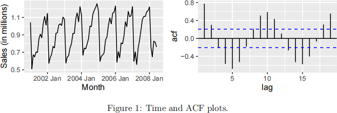
f The ACF plot shown to the right of Figure 1 does not match with the time
plot given.
[Total: 20 marks]
2 Figures 2 and 3 show the time, seasonal, and subseries plots for quarterly sales (in millions of dollars) from food and beverage services in New Zealand over the period
1995 Q3–2020 Q4.
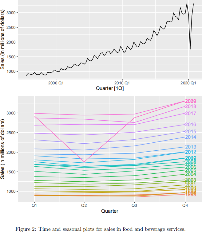
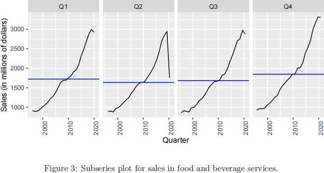
a Using Figures 2 and 3, describe the sales data for food and beverage services in New Zealand . Your answer must refer to information obtained from all three plots. [9 marks]
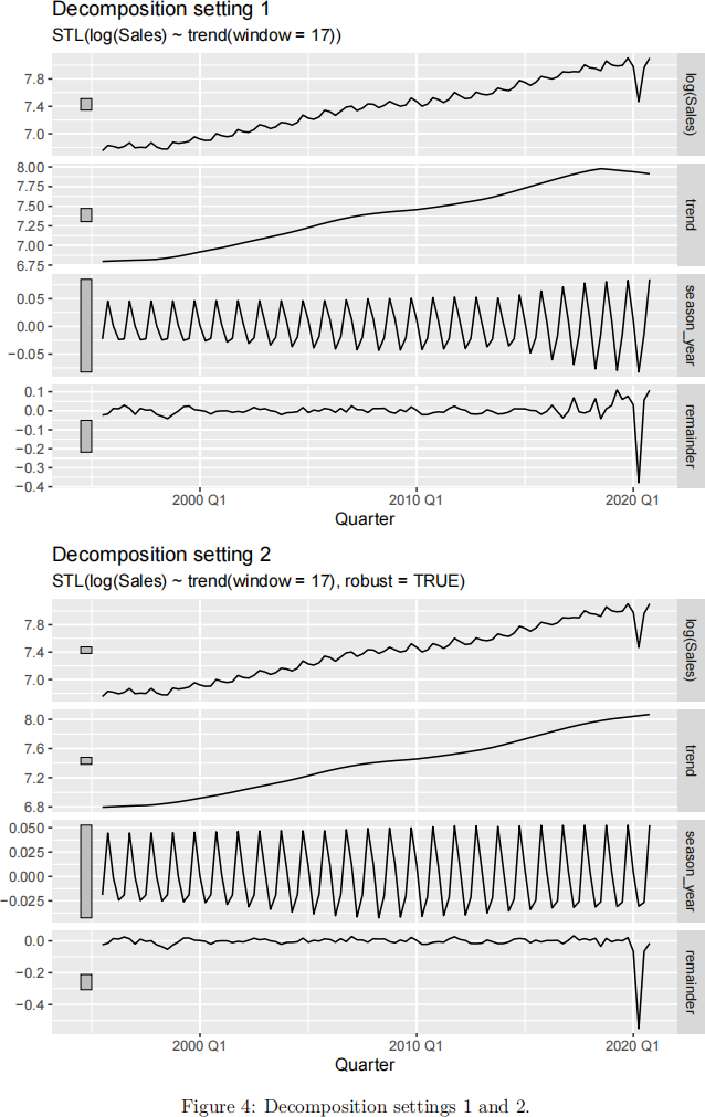
b The sales time series is decomposed into its components using two different settings. The estimates of the decomposition are shown in Figure 4.
Comment on
• what is plotted in all eight panels of Figure 4;
• the behaviour of each component over time;
• the effect of using robust = TRUE.
Which setting would you consider appropriate for this time series?
[16 marks] [Total: 25 marks]
3 Figure 5 shows the number of employees’ in food and beverage stores in the US over the period January 1990–March 2021.
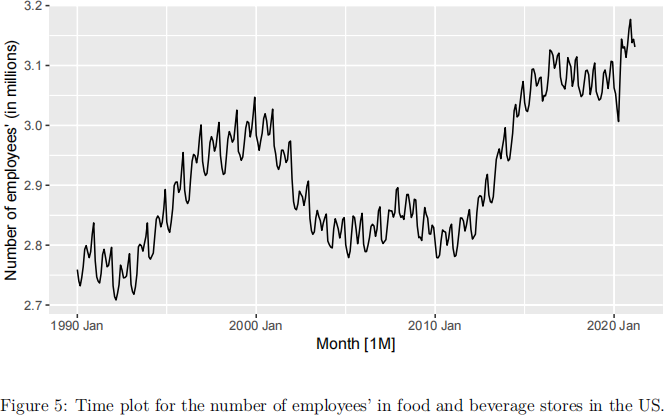
a Briefly comment on the main features that you can observe in this time series?
Can you identify any unusual observations? [4 marks]
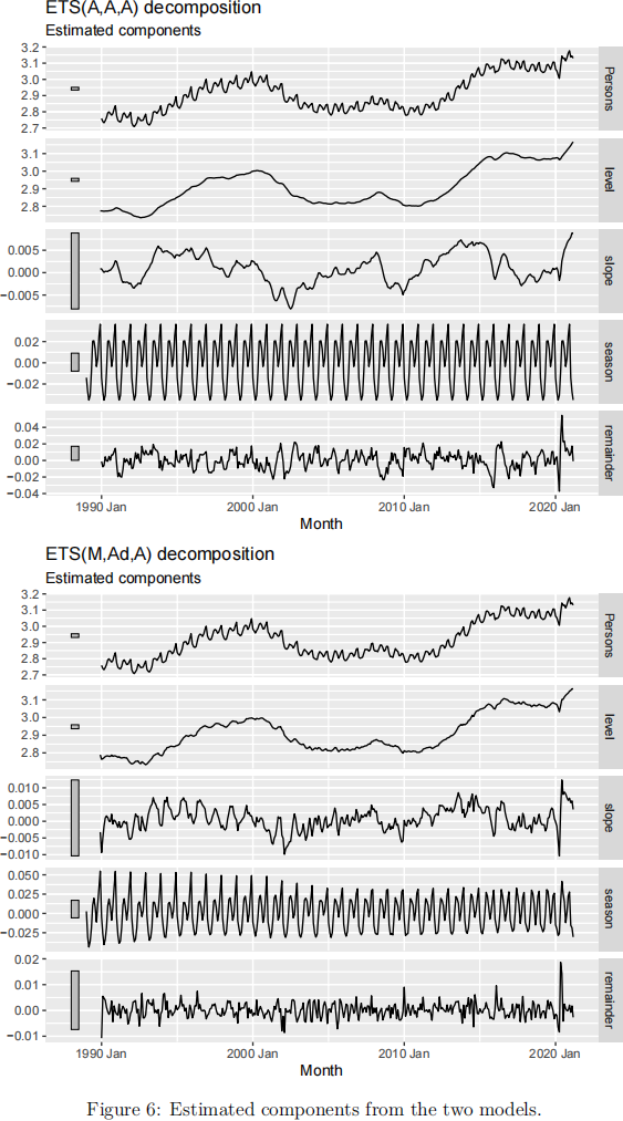
b The R code below is used to fit two models to the employees’ data shown in Figure 5 and to extract summary output from each model.
The estimated components for the two models are shown in Figure 6. Use this information to answer questions 3(b)i–3(b)vi.
fit <- employees_food %>%
model(
additive = ETS(Persons ~ trend("A")),
damped = ETS(Persons ~ trend("Ad"))
)
fit %>% select(additive) %>% report()
## Series: Persons
## Model: ETS(A,A,A)
## Smoothing parameters:
## alpha = 0.253
## beta = 0.0545
## gamma = 0.000104
##
## Initial states:
## l b s1 s2 s3 s4 s5 s6
## 2.77 0.000889 0.0364 0.0254 0.00395 -0.00354 0.0128 0.0207
## s7 s8 s9 s10 s11 s12
## 0.0205 -0.00885 -0.0308 -0.0352 -0.0273 -0.014
##
## sigma^2: 1e-04
##
## AIC AICc BIC
## -1156 -1154 -1089
fit %>% select(damped) %>% report()
## Series: Persons
## Model: ETS(M,Ad,A)
## Smoothing parameters:
## alpha = 0.754
## beta = 0.217
## gamma = 0.24
## phi = 0.879
##
## Initial states:
## l b s1 s2 s3 s4 s5 s6
## 2.79 -0.00323 0.0548 0.0333 0.0119 -0.0112 0.00827 0.0197
## s7 s8 s9 s10 s11 s12
## 0.0106 -0.0194 -0.0363 -0.0435 -0.0308 0.00272
##
## sigma^2: 0
##
## AIC AICc BIC
## -1286 -1284 -1215
Note: The ![]() ̂ 2 for the damped model appears in the summary output as zero due to the rounding.
̂ 2 for the damped model appears in the summary output as zero due to the rounding.
i Describe the differences between the two model specifications. [5 marks]
ii Describe the estimated components shown in Figure 6 for the ETS(A,A,A) model. Explain how they are related to the estimated parameters. [4 marks]
iii Considering the names of the R objects created above for this question, write R code to assess the fit of the additive model. [6 marks]
iv What modifications would you make to the R code written in 3(b)iii to assess the fit of the damped model? [3 marks]
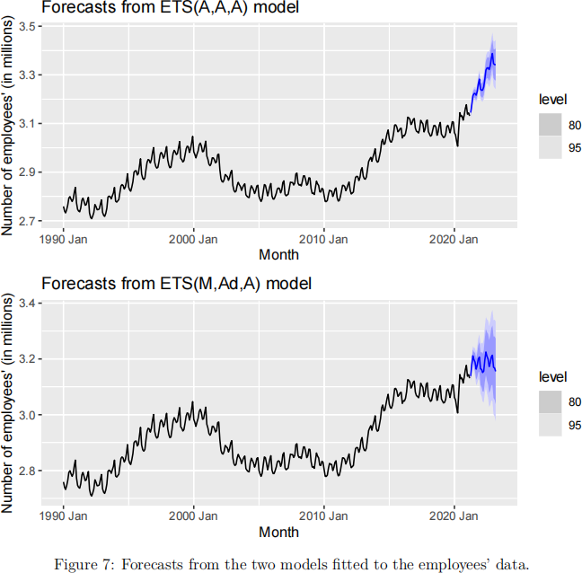
v Figure 7 shows forecasts from the two fitted models. Based on these forecasts, which model would you choose for the given data. Give reasons for your selection. [6 marks]
vi Write down the equations for the model you have chosen in 3(b)v. [5 marks] [Total: 33 marks]
4![]() Consider the employees’ time series data used in Question 3. The following R code creates three new variables.
Consider the employees’ time series data used in Question 3. The following R code creates three new variables.
employees_food %>%
mutate(diff_persons = difference(Persons),
sdiff_persons = difference(Persons, 12), diff_sdiff_persons = difference(difference(Persons, 12)))
Figures 8 and 9 show time, ACF, and PACF plots for the original employees’ time series and the new variables constructed in the R code above.
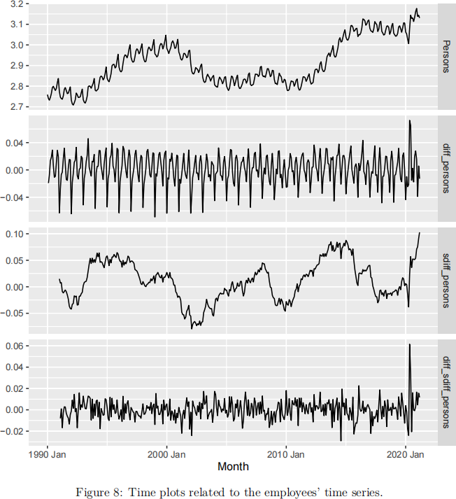
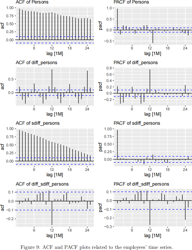
a Use Figures 8 and 9 to find an appropriate differencing to obtain a stationary time series for employees’ data. Give reasons for your selection. [6 marks]
b The R code below is used to fit three models to the employees’ data and extract summary output from each model.
Consider the model for your choice of differencing in 4a to answer questions 4(b)i–4(b)iii.
fit <- employees_food %>%
model(arima1 = ARIMA(Persons ~ pdq(d = 1) + PDQ(D = 0), stepwise = FALSE),
arima2 = ARIMA(Persons ~ pdq(d = 0) + PDQ(D = 1), stepwise = FALSE),
arima3 = ARIMA(Persons ~ pdq(d = 1) + PDQ(D = 1), stepwise = FALSE))
fit %>% select(arima1) %>% report()
## Series: Persons
## Model: ARIMA(4,1,0)(0,0,2)[12]
##
## Coefficients:
## ar1 ar2 ar3 ar4 sma1 sma2
## 0.0810 -0.181 -0.1915 -0.1115 0.7616 0.5468
## s.e. 0.0547 0.051 0.0511 0.0539 0.0602 0.0572
##
## sigma^2 estimated as 0.0001507: log likelihood=1112
## AIC=-2210 AICc=-2210 BIC=-2182
fit %>% select(arima2) %>% report()
## Series: Persons
## Model: ARIMA(2,0,1)(1,1,2)[12]
##
## Coefficients:
## ar1 ar2 ma1 sar1 sma1 sma2
## 1.9639 -0.965 -0.9190 -0.737 0.121 -0.6135
## s.e. 0.0221 0.022 0.0319 0.168 0.155 0.0936
##
## sigma^2 estimated as 6.55e-05: log likelihood=1231
## AIC=-2449 AICc=-2448 BIC=-2421
fit %>% select(arima3) %>% report()
## Series: Persons
## Model: ARIMA(0,1,0)(0,1,2)[12]
##
## Coefficients:
## sma1 sma2
## -0.5482 -0.1959
## s.e. 0.0595 0.0602
##
## sigma^2 estimated as 6.721e-05: log likelihood=1223
## AIC=-2440 AICc=-2440 BIC=-2428
i Describe the relationship between the relevant ACF and PACF plots given in Figure 9 to the orders estimated in the ARIMA model. [5 marks] ii Write down the estimated model using the backward shift operator. [3 marks]
iii Use the information given below to compute a 1-step-ahead forecast and its 95% prediction interval for the model written in 4(b)ii. [8 marks]
[Total: 22 marks]
Information about arima1 model
## # A tsibble: 15 x 3 [1M]
## Month Persons .resid
## <mth> <dbl> <dbl>
## 1 2020 Jan 3.06 -0.0124
## 2 2020 Feb 3.05 -0.00915
## 3 2020 Mar 3.03 -0.0222
## 4 2020 Apr 3.01 -0.0302
## 5 2020 May 3.08 0.0590
## 6 2020 Jun 3.14 0.0306
## 7 2020 Jul 3.13 -0.0202
## 8 2020 Aug 3.13 0.0261
## 9 2020 Sep 3.11 0.00132
## 10 2020 Oct 3.13 0.0111
## 11 2020 Nov 3.16 0.0165
## 12 2020 Dec 3.18 0.0164
## 13 2021 Jan 3.14 -0.0125
## 14 2021 Feb 3.14 0.0212
## 15 2021 Mar 3.13 0.00427
Information about arima2 model
## # A tsibble: 15 x 3 [1M]
## Month Persons .resid
![]()
![]()
![]() <dbl>
<dbl>

 ## 1
## 1
## 2
## 3
## 4
## 5
## 6
## 7
## 8
## 9
## 10
## 11
## 12
## 13
## 14
## 15
Information about arima3 model
## # A tsibble: 15 x 3 [1M]
## Month Persons .resid
![]()
![]()
![]() <dbl>
<dbl>


![]() ## 1
## 1
## 2
## 3
## 4
## 5
## 6
## 7
## 8
## 9
## 10
## 11
## 12
## 13
## 14
## 15
2023-06-14
Time Series Forecasting for Data Science