ECMT2150 INTERMEDIATE ECONOMETRICS Week 7 Tutorial
Hello, dear friend, you can consult us at any time if you have any questions, add WeChat: daixieit
ECMT2150 INTERMEDIATE ECONOMETRICS
Week 7 Tutorial - Heteroskedasticity
Stata 1 (Wooldridge, Wadud and Lye Exercise C2 Chapter 9)
The Australian version of the Deal or No Deal television game show, in which contestants sequentially open cases to reveal prizes, was shown in Australia between 2004 and 2013. The game show is still on TV in the US.
The data used in this exercise were obtained from televised episodes of Deal or No Deal in Australia in the period 2 February 2004 to 25 November 2005. The 232 games in this sample were regular games without special prizes or ‘super cases’ . The details of the game can be widely found on the Internet and a number of scholarly papers have been written to examine the nature of the decisions made by the contestants. Or you can ask a friend who has enough free time to have watched the show.
The data set DEAL.dta contains a number of variables. Either the offer is accepted because the contestant takes the ‘Deal’ from the bank (no_deal = 0), or the contestant opts for ‘No Deal!’ (no_deal = 1) and they keep the case they have with the unknown amount. The variable winnings is either the value of the offer they take from the bank or, if they take what was in their case, the value of own_case. Other variables in the data set include doff, the change in the offer made since the last round; davg, the change in the average value of the unopened cases from the last round; and num_left, the number of unopened cases.
a) Use the variable winnings as the dependent variable with doff, davg and num_left as regressors. Report the results in the usual way.
b) Obtain the OLS residuals, u it and regress these on all of the independent variables. Explain why you obtain R2 = 0.
c) Apply the modifed White test for heteroskedasticity as outlined in lectures. Report the F- stat and the p-value. Use the p-value to reach your conclusion. What do you conclude?
d) For the sake of completeness, use the Breusch Pagan test for heteroskedasticity as well. Is there any change in your conclusion from c)?
e) Re-estimate the model but now report the heteroskedasticity-robust standard errors. Discuss any important differences in the results.
f) In light of your findings, do the producers of this show have any control over the winnings by use of these variables?
Q1 (Wooldridge Problem 2 Chapter 8)
Consider a linear model to explain monthly beer consumption:
beeT = F0 + F1 inc + F2pTice + F3 educ + F4female + u
E(u|inc, pTice, educ, female) = 0
Var(u|inc, pTice, educ, female) = a2 inc2 .
Write the transformed equation that has a homoskedastic error term. Show that the transformed error term is homoscedastic.
Q2 (Wooldrige, Wadud and Lye Chp 9 Q4)
The following equation was estimated for the first semester of undergraduate students based on their semester results in a university in New South Wales:
markavg = −11.016 + .516 sthours + .812 atar + .551 female + 3.112 mode
(2.586) (.0578) (.0326) (.7966) (1.541)
[2.565] [.068] [.0346] [.797] [1.412]
n=456, R2 =.74.
Here, markavg is the average mark obtained by each student in the subjects completed in the semester, sthours is the total number of hours of study of each student over the semester, atar is each student’s individual ATAR score, female is a gender dummy, and mode is a dummy variable equal to unity if the student completed the semester as an on-campus student. The usual and heteroskedasticity-robust standard errors are reported in parentheses and brackets, respectively.
a) Do the variables sthours, atar, female and mode have the expected estimated effects? Which of these variables are statistically significant at the 5% level? Does it matter which standard errors are used?
b) Test the hypothesis H0 : Fatar = 1 against the two-sided alternative at the 5% level, using both standard errors. Describe your conclusions.
c) Test whether there is a positive impact of a student’s mode of learning as on-campus. Does the significance level at which the null can be rejected depend on the standard error used? Explain your answer.
Q3 (Wooldridge Chapter 8, Problem 5)
The variable smokes is a binary variable equal to one if a person smokes, and zero otherwise. Using the data in SMOKE, we estimated a linear probability model for smokes:
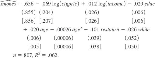
The variable white equals one if the respondent is white, and zero otherwise; the other independent variables are defined in Example 8.7. Both the usual and heteroskedasticity- robust standard errors are reported.
a) Why should we use heteroskedasticity-robust standard errors when estimating this model? In this particular example, are there any important differences between the two sets of standard errors?
b) Holding other factors fixed, if education increases by four years, what happens to the estimated probability of smoking?
c) At what point does another year of age reduce the probability of smoking?
d) Interpret the coefficient on the binary variable restaurn (a dummy variable equal to one if the person lives in a state with restaurant smoking restrictions).
e) Person number 206 in the data set has the following characteristics:
cigpric =67.44, income=6,500, educ=16, age=77, restaurn=0, white=0, and smokes=0. Compute the predicted probability of smoking for this person and comment on the result.
Extra question if you want more practice
1. (Wooldridge Computer Exercise C4 Chapter 8)
Use VOTE1 for this exercise.
(i) Estimate a model with voteA as the dependent variable and pTtystTA, demoCA, log (expendA), and log (expendB) as independent variables. Obtain the OLS residuals, u换it and regress these on all of the independent variables. Explain why you obtain R2 = 0.
(ii) Now, compute the Breusch-Pagan test for heteroskedasticity. Use the F statistic and
report the p-value.
(iii) Compute the special case of the White test for heteroskedasticity, again using the F
statistic. How strong is the evidence for heteroskedasticity now?
2023-06-08