ECMT6007/ECON4954 Analysis of Panel Data
Hello, dear friend, you can consult us at any time if you have any questions, add WeChat: daixieit
ECMT6007/ECON4954 Analysis of Panel Data
Answer Key to Mid-semester Exam, Semester 1, 2022
❼ INSTRUCTIONS
– Answer all questions by yourself. Make sure you read, understood and comply with the University of Sydney Academic Honesty in Coursework Policy 2015 and the Academic Honesty Procedures 2016.
– You can type your answer (using MS word or Latex editors), or write down on papers and scan the papers into a single answer book as a PDF file; in case you are unable to scan the papers, you may take photos of them and arrange them into a single answer book as a PDF file. Taking photos is not recommended as the photo quality may not be good enough. Either way, please make sure your answer is clear and legible.
– Set the file name of your PDF answer book as ECMT6007-SID or ECON4954-SID; Submit the PDF answer book via Turnitin on Canvas. Do not submit by emails.
Question 1 [100 marks] The questions are based on empirical studies of the effect of trade unions on labour market outcomes. Recent empirical research on this topic has focused on panel survey data and methods. A primary focus of the research is the effect of unions on a worker’s ln(wage) - the natural log of the real hourly wage - and the key explanatory variable is union status which is an indicator of whether the worker is a union member. In these studies, the cross-sectional observational unit is an individual worker (each with a unique value for the identifier variable id) with annual measures of the variables based on a survey. The common model specification in the literature is
ln(zageit) =80 + 81wnipnit + 82 edwcit + 83 ergetit + 84 ergetit(2)
+ 85manwfit + ai + wit (1)
where the variables are:
i = person identifier (the cross-sectional units with 110 individuals in the survey) t = time period identifier (the panel survey covers 8 time years, 2010 to 2017)
ln(zageit) = ln(real hourly wage) of worker i in year t
wnipnit = 1 if worker i is a union member in year t (= 0 otherwise)
edwcit = years of completed education of worker i in year t
ergetit = years of labour market experience of worker i in year t
manwfit = 1 if worker i is employed in manufacturing in year t
twtit = 1 if worker i lived in a rural area in year t
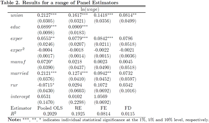
Consider a panel survey where i = 110 individual workers are surveyed annually for u = 1, ..., 8 time periods (from 2010 to 2017). Summary Statistics are reported in Table 1 below. The results for a range of panel estimators are presented in Table 2 below.
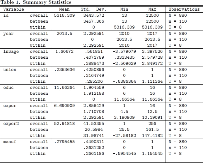
1. Version A [10 marks] Based on Table 1, why is the within variation of the variable id equal to zero? Why is the between variation of the variable year equal to zero? Briefly explain.
Since i is the person identifier, it does not change over time so that the within variation of the variable id equal to zero. For each year, t does not vary across individuals so that the between variation of the variable year equal to zero.
Version B [10 marks] Based on Table 1, is the sample a short or long panel, a balanced or unbalanced panel? What is the primary nature of the variation in the variable edwcit? Briefly explain.
It is a short panel as n = 110 and T = 8 so that n > T ; Balanced as N = n | T (no missing observations). The within variation in the variable edwcit is zero since the year of schooling remains the same after an individual graduated (from a high school or a college).
2. Version A [10 marks] Give two examples, with a justification, of factors captured by the term wit .
Note that wit is the idiosyncratic error that varies across i and over u; also wit captures unobserved factors that affects wages. Examples include shocks to health, and external job offers.
Version B [10 marks] Give two examples, with a justification, of factors captured by the term ai .
Note that ai captures the time-invariant individual heterogeneity that varies across i and does not change over u; also ai captures unobserved factors that affects wages. Examples include ability, race, and gender.
Note: a reasonable justification is required for full credit.
3. Version A [10 marks] What is the interpretation of 82 in model (1)? Be precise in your statement of the interpretation.
As the coefficient of edwcit , 82 captures the effect on ln(zageit) of education level, holding other factors constant.
Version B [10 marks] What is the interpretation of 81 in model (1)? Be precise in your statement of the interpretation.
As the coefficient of wnipnit , 81 captures the effect on ln(zageit) of being a union member, holding other factors constant.
4. Version A [10 marks] Under what conditions is the Pooled OLS (POLS) estimator unbi- ased? Do you think they are satisfied in this empirical study? Explain your reasoning.
For the Pooled OLS (POLS) estimator to be unbiased, MLR1 - MLR4 must be satisfied (need to be specific to the empirical example in the question):
❼ MLR1 - the model is correctly specified as a linear model in (1);
❼ MLR2 - the sample is random (or i.i.d);
❼ MLR3 - no perfect collinearity;
❼ MLR4 - regressors are exogenous,
They are unlikely to hold in this application. Especially, MLR4 (exogeneity) is typically violated as education is correlated with ability, which is part of ai .
Version B [10 marks] Under what conditions is the Pooled OLS (POLS) estimator consis- tent and efficient? Do you think they are satisfied in this empirical study? Explain your reasoning.
For the Pooled OLS (POLS) estimator to be consistent, we need MLR1 - MLR4 above; for efficiency, besides MLR1 - MLR4, we also need
❼ MLR5 - homoskedasticity and no autocorrelation in the error (ai+ wit),
Again, MLR4 (exogeneity) is typically violated as education is correlated with ability, which is part of ai . Also, MLR5 is impossible with the presence of ai except that ai is constant.
5. Version A [10 marks] What, if any, are the advantages of the random effects (RE) esti- mator over the pooled OLS estimator for 81 ? Briefly explain.
If ai is a fixed effect, both RE and POLS estimators are inconsistent. If ai is a random effect, both RE and POLS estimators are consistent. The main advantages of the random effects (RE) estimator over the pooled OLS estimator is that RE is more efficient than POLS as it adjusts for autocorrelation in the error (ai+ wit) due to ai . Note that the s.d. of POLS calculated using the regular formula is invalid; the robust version should be used to estimate the s.d. In addition, POLS ignores the unobserved individual heterogeneity (in terms of level/intercept).
Version B [10 marks] As shown in Table 2, the First Difference (FD) estimate of 81 is significantly lower than the FE and RE estimates of 81 . The FD estimate of 81 also has a larger standard error than the FE and RE estimates. Provide a possible explanation for these differences in estimation results.
Based on the first-differenced equation, 81 captures the effect of △wnipnit on △ ln(zageit) which tends to be small as changing union status does not directly affect wage (in the same year). Since wnipnit is the union indicator that does not change frequently, the within variation of △wnipnit is typically very small (with a high autocorrelation) so that the FD estimate of 81 has a larger standard error than the FE and RE estimates.
6. Version A [10 marks] Express the sample regression model for each individual i; Using matrix with summation notation, show the First Difference (FD) transformed equation and the FD estimator.
For i, define the matrices
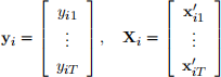
where yi = (yi1 , | | | , yi8)\ is the vector of regressand and Xi the matrix of regressors in equation (1) including the intercept. Equation (1) can be expressed as
yi = Xi8 + ai4 + ui
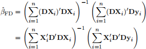
where 4 is a 8 来 1 vector of 1’s and ui = (wi1 , | | | , wi8)\ , and 8 = (81 , | | | , 85 )\ . The First Difference (FD) transformed equation is
Dyi = DXi8 + Dui
where D is the FD matrix; Alternatively, you may use the FD operator △ and get △yi = △X![]() 8 + △ui . the FD estimator can be expressed as
8 + △ui . the FD estimator can be expressed as
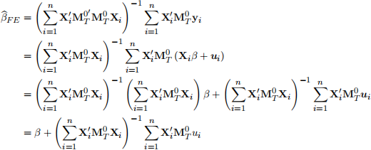
Version B [10 marks] Using matrix with summation notation, show the Fixed Effect (FE) transformed equation and the FE estimator. Decompose the FE estimator into 8 + estimation error.
Again, the model can be expressed as yi = Xi8+ai4+ui . The Fixed Effect (FE) transformed equation is
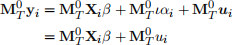
where MT(0) = IT | ![]() 44\ is the centering matrix and MT(0)4ai = 0. The FE estimator is the GLS applied to the transformed model:
44\ is the centering matrix and MT(0)4ai = 0. The FE estimator is the GLS applied to the transformed model:

The FE estimator can be decomposed as
7. Version C [10 marks] List the assumptions for the estimator in Part (6) to be consistent, and show that the estimator is consistent under these assumptions.
For the FD estimator estimator 8ˆFE to be consistent for 8, besides the regular assumptions on linear regressions
❼ MLR1 (linear model): y = 80 + X8 + aL + u
❼ MLR2 (random sample): yi = 80 + Xi8 + aiL + ui where cross sectional units are
independent.
❼ MLR3 (no perfect collinearity),
the exogeneity assumption MLR4 needs modification:
❼ MLR4 (exogeneity): and E(ui这Xi) = 0.
To show consistency of 8ˆFD , decompose 8ˆFD

By the LLN,
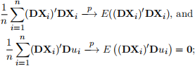
where the second line follows from the strict exogeneity condition.
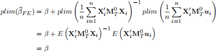
For the FE estimator, the assumptions for consistency are the same as those for the FD estimator. To show consistency of ![]() FE , using the results in (7),
FE , using the results in (7),
8. Version A [10 marks] Calculate the degrees of freedom for the POLS, FE, RE and FD estimators in Table 2, respectively.
Note: in equation (1), the number of slope coefficients k = 5 while k = 7 in Table 2; either one is ok. Also note that edwc is time-invariant in this application so that, for the FD and FE, the effective number of slope coefficients becomes k = 4 in equation (1) and k = 6 in Table 2. The degrees of freedom for the POLS, FE, RE and FD estimators in Table 2
❼ POLS: nT | k | 1 = 880 | 5 | 1 = 874 or nT | k | 1 = 880 | 7 | 1 = 872
❼ FD: nT | k | n = 880 | 4 | 110 = 766 or nT | k | n = 880 | 4 | 110 = 764
❼ FE: nT | k | n = 880 | 4 | 110 = 766 or nT | k | n = 880 | 4 | 110 = 764
❼ RE: nT | k | 1 | 2 = 880 | 5 | 1 | 2 = 872 or nT | k | 1 | 2 = 880 | 7 | 1 | 2 = 870
Version B [10 marks] The RE estimate can be connected to two other estimates. Briefly explain the intuition behind this relation. Is it confirmed by the results in Table 2? The RE estimate can be connected to the POLS and FE/Within estimates: for the transformed equation
yit | 9y¯i = (xit | 9 ![]() i) 8 + (wit\ | 9
i) 8 + (wit\ | 9 ![]() i)
i)
the RE moves towards the POLS as 9 书 0 and become the POLS when 9 = 0, which is appropriate when 7α(2) = 0 and the POLS is optimal; the RE moves towards the FE as 9 书 1 and become the FE estimate when 9 = 1, which is consistent when ai indeed is a fixed
effect. This is confirmed in Table 2 for all slope coefficients except the one for edwc which is not available with FE estimation.
9. [10 marks] Propose a hypothesis test to decide whether the RE estimator or the FE esti- mator is more appropriate for this application. Please write down the null and alternative hypotheses, propose the test statistic and the distribution it follows, and state the deci- sion rule.
The null and alternative hypotheses are
The Wu-Hausman’s test statistic is

which is asymptotically x2 (r) distributed under H0; Note that r = 6 based on Table 2. With wH calculated, H0 is rejected at level a if wH > xα(2) (r) or the p-value is smaller than the significance level (such as 5% or 1%) .
A. with a p-value at 0.126, H0 is rejected at 10%.
B. with a p-value at 0.0025, H0 can not be rejected at 1%.
10. Version C [10 marks] Based on Table 2 and the answer in Question (9), what effect does union membership have on the expected wage? What is the best estimate of the effect and why?
Since it is believed that edwc is endogenous, only the FD and FE estimators are consistent; also, the FD estimate of 81 is significantly lower than the FE and RE estimates, the FE estimator is preferred. Note: if the null hypothesis is not rejected as in (9), the RE estimator is also acceptable. Based on the FE estimate of 81 (0.1418), on average, the wage is expected to be 14.18% higher with a union membership, holding other factors constant.
2023-05-20