General instructions:

•    This is an individual assignment.

•    The assignment will be marked out of 25 marks and is worth 25% of your overall grade for this course.

•     Please submit your assignment online through Canvas by the due date as a PDF document.

•     Proper referencing (APA style or other referencing style used by a major Accounting or Finance journal) must be used if you use external sources.

•     Late submissions will lose 5 marks for each day they are late.

Background:

This assignment involves quantitative data analysis. The purpose of the assignment is to help you familiarise yourself with techniques and tools commonly used for data              manipulation and quantitative analysis in accounting and finance research.

The theme of this assignment is based on a study by Graham and Leary (2018), which  investigates corporate cash holdings . It may be helpful to refer to this study for context, although this is not explicitly required in order to complete this assignment. The full       reference for the study is given below and a link is also provided through the Week 2     reading list on Canvas :

Graham, J. R., & Leary, M. T. (2018). The evolution of corporate cash . The Review of Financial Studies, 31(11), 4288-4344.

You are provided with two datasets (both CSV file and SAS Data Set versions of the data are provided on Canvas) :

1.  “fundamentals” containing firm fundamentals/financial reporting data

2.  “market” containing stock return and other trading information.

The source of the data is CRSP and Compustat. The data is provided at the yearly level. It covers 70 years from 1950 to 2019. In total, there are 156,823 firm-year

observations. Both of the datasets cover the same time period and the same firms. The

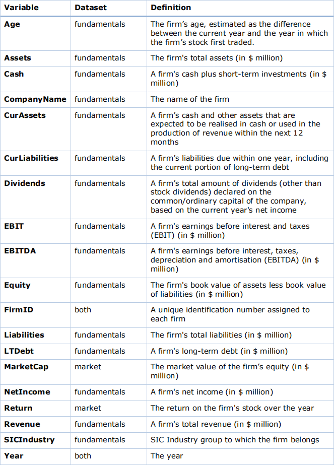
variables included in the data are defined in Table 1 below .

Table 1 Variables and definitions

Required statistical software:

To do this assignment, you will need to use statistical software. You are free to use         whichever software package you like, but the recommended software is either SAS or     Stata. (Excel is unlikely to be sufficient to complete all parts of the assignment). SAS      and Stata are installed on many university computers. You can also access them through your personal computer through FlexIT (see instructions provided previously).

Detailed instructions:

You need to use the two datasets provided to perform a series of data manipulation and analysis steps as detailed below . Most (but not all) of the steps have required output     that you need to include in your assignment submission as indicated . Checks are           provided in many of the steps so you can make sure your analysis is correct.

In your submission, make sure that you include all the required output under each step. You should also include any code you use in your analysis as an appendix. Your             assignment should be submitted as a pdf file.

Steps to follow:

1.  Merge/join the two datasets together by firm and year using the identifier, “FirmID”, and “Year” .

Required output to include in submission: None.

Check: The merged dataset should have 156,823 observations and 19 variables. (0 marks)

2.  Create six new variables called “CashRatio”, “DARatio”, “ROA”, “DivPayer”, “LnAssets” and “LnAge” as follows :

CashRatio =

→ This is the firm’s cash holdings as a proportion of assets.

DARatio  =

→ This shows a firm’s long-term debt as a proportion of total assets.

ROA =

→ This is the EBITDA return on assets ratio.

1 if Dividends > 0

0 otherwise

→ This is a dummy variable equal to 1 if a firm is a dividend payer (has     declared dividends greater than zero during the year), and zero otherwise.

LnAssets = ln(Assets ∗ 1,000,000)

→ This is the natural logarithm of a firm’s total Assets .

LnAge = ln(Age)

→ This is the natural logarithm of a firm’s age in years.

Required output to include in submission: None

Check: The value of the above variables for the firm with FirmID 4115 in year

2005 should be :

(0 marks)

3.  Produce a table showing summary statistics for the variables: Age, Assets, Cash, EBITDA, Equity, Liabilities, LTDebt, MarketCap, NetIncome, Return, Revenue,     CashRatio, DARatio, DivPayer and ROA . You should include the following             statistics:

-    Number of observations

-    Mean

-    Standard deviation

-    Minimum

-    Maximum

Required output to include in submission: A table displaying the summary statistics as indicated above .

Check: Below is an excerpt from the results:

(1 mark)

4.  Produce a correlation matrix for the variables: Age, MarketCap, Return, CashRatio, DARatio and ROA .

Required output to include in submission: A table/matrix that displays the correlation coefficients and an indication of the statistical significance for each pair of variables (eg p-values).

Check: Below is an excerpt from the results:

(1 mark)

5.  Carry out a t-test for the difference in means to test the following null hypothesis:

H0 : There is no difference in the cash ratio between firms that pay a dividend and firms that don’t pay a dividend.

Assume unequal variances between the two groups when carrying out the t test. Required output to include in submission: Display the results of your t test  (including difference in mean cash ratio between the two groups and statistical   significance) in a table. Write one sentence summarising your conclusion in        relation to the null hypothesis.

Check: The difference in the means between the two groups should be 0.1013. (2 marks)

6.  Produce a line chart that shows how the annual cash ratio varies over the sample period for firms as a whole. The chart should show two series:

a.  The equally weighted average cash ratio across all firms by year.

b.  The average cash ratio by year, value weighted across firms according to firms’ market capitalisation each year.

A hypothetical example demonstrating the calculations for a single year with 3 firms is shown below:

Equally weighted average = = 0.267

Value weighted average = × 0. 10 + × 0.25 + × 0.45 = 0.32

Required output to include in submission: A chart showing the two series as described above. Note: you can create the chart in SAS/Stata directly if you like.

However, if you prefer you can also export the required data to a csv file, open it in Excel and then create the chart in Excel.

Check: A plot of the equally weighted series is shown below:

ewCashRatio

0.30

0.25

0.20

0.15

0.10

0.05

0.00

(2 marks)

7.  Calculate a new variable called “LagReturn” . This is the return on a firm's stock over the previous year.

Required output to include in submission: None

Important: The LagReturn variable should only have a value for observations where there is a return available for the previous year for the same firm .        Therefore:

•    the LagReturn variable will have a missing value for the observation corresponding to the first year for each firm

•     if, for a given observation, there is no data available for the previous year for that firm, then the LagReturn variable will have a missing value for     that observation.

Check: The value of LagReturn for the firm with FirmID 5540 in year 2002 should be 0.04469. The dataset should have 15,964 observations with missing values for

LagReturn.

(0 marks)

8.  Run the following regressions :

Model 1 : CasℎRatioi,t  = F0  + F1 LnAssetsi,t  + ei,t

Model 2 : CasℎRatioi,t  = F0  + F1 LnAssetsi,t  + F2 LnAgei,t  + F3 DARatioi,t  + F4 DivPayeTi,t  + F5 LagRetuTni,t  + ei,t

Model 3 : CasℎRatioi,t  = F0  + F1 LnAssetsi,t  + F2 LnAgei,t  + F3 DARatioi,t  + F4 DivPayeTi,t  + F5 LagRetuTni,t  + SIC IndustTy GToup Fixed Effects + ei,t

Model 4 : CasℎRatioi,t  = F0  + F1 LnAssetsi,t  + F2 LnAgei,t  + F3 DARatioi,t  + F4 DivPayeTi,t  + F5 LagRetuTni,t  + YeaT Fixed Effects + ei,t

Model 5 : CasℎRatioi,t  = F0  + F1 LnAssetsi,t  + F2 LnAgei,t  + F3 DARatioi,t  + F4 DivPayeTi,t  + F5 LagRetuTni,t  + SIC IndustTy GToup Fixed Effects + YeaT Fixed Effects + ei,t

Required output to include in submission:

A single table displaying the results of each of the above regression models. The table should show the following for each model :

-    Coefficient estimates. (Note: for models that include fixed effects,           coefficient estimates for the fixed effects don’t need to be shown in the   table. Instead, simply indicate whether or not the fixed effects are          included in a given model . The value for the intercept also does not need to be shown in the table .)

-    Standard errors or t-statistics for the coefficient estimates.

-    Indication of the statistical significance of each coefficient estimate (eg stars).

-    R-squared.

Interpret the coefficient estimates of:

-    F3   and F4   in Model 3.

Describe what the purpose is of including industry and year fixed effects. Check: The coefficient estimate of F1   should be in -0.01525 Model 1 and the coefficient estimate of F5   should be 0.00887 in Model 5 .

(4 marks)

9.  Come up with your own research question related to the topic of corporate cash holdings and carry out some quantitative analysis to answer your research         question.

This question is a chance for you to apply the quantitative analysis skills and     techniques covered in this course to carry out your own small piece of research. You can choose any research question you like related to the above topic. You   then need to design and carry out some quantitative analysis to answer this      research question.

If you wish to add more data, you can, but this is NOT required. You can get full marks by using only the data provided for the assignment .

You will be graded based on the quality of your analysis and how well you present and interpret it. As a guide for how much work is required, your answer for this    question should be no longer than 5 pages.

Required output to include in submission:

Your answer should include the following sections:

Introduction/Research question

Decide on a research question related to the above topic. Describe your research question and include in your description an appropriate null hypothesis and          alternative hypothesis. Explain the purpose of your research question (ie why it is an interesting and relevant question) .

Data and Methodology

Clearly describe your approach to the analysis and the methodology you are applying, including statistical tests, econometric models etc as appropriate . Provide some information about the data (eg descriptive statistics).

Results/Conclusion

Present the results of your analysis and interpret these results in the context of your research question. Provide a conclusion to answer your research question. Explain whether or not the null hypothesis can be rejected in favour of the        alternative hypothesis. Provide some discussion of limitations of your research and/or potential opportunities for further research where relevant.

Note: Presentation is important for this question . You should pay attention to       factors such as structure and formatting, presenting important information clearly and use of tables/charts where appropriate . Don’t forget to reference if you refer to external sources .

(15 marks)

Detailed marking guide

For questions 1-8, you will get full marks if you get the right answer. No marks are       awarded for presentation, so you can just copy and paste your outputs from Stata/SAS . However, make sure it is clear and don’t forget to provide the short sentence answers   where needed.

10 marks (total for questions 1-8)