ECMT3150: Assignment 1 (Semester 1, 2023)
Hello, dear friend, you can consult us at any time if you have any questions, add WeChat: daixieit
ECMT3150: Assignment 1 (Semester 1, 2023)
Due: 5pm, 21 March 2023 (Tuesday)
1. [Total: 24 marks]
Note: Please append your R codes (as a separate .R file) for part (g) while you submit the assignment.
Let Xi denote the log-price of a stock, Cherry Inc. (code: CRRY), by the end of trading day i, and let AXi := Xi _ Xi━1; thus AXi is the log-return on trading day i (i.e., over period (i _ 1;i]).
Assume {Xi}![]() ≥〇 follows the AR(1) model:
≥〇 follows the AR(1) model:
 (1)
(1)
where ui ~ iid normal with mean 0 and variance 72 .
Let {Fi}i≥〇 be the natural filtration generated by {ui}i≥〇 .
(a) [2 marks] Express AXi in terms of Xi━1 and ui .
(b) [2 marks] Compute E(AXi|Fi━1).
(c) [2 marks] Compute Var(AXi|Fi━1).
(d) [2 marks] What is the condition on o〇 and o1 such that {AXi}i≥1 is a martingale difference sequence?
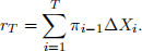
A trading strategy is defined by {π i}i≥〇, where π i is measurable with respect to Fi . Specifi- cally, π i represents the number of CRRY shares a trader buys at the start of day i. The log-return due to the trading strategy over period (0;T] is given by
(e) [4 marks] Alice invested in a share of CRRY using a buy-and-hold strategy, with π i 三 1 for all i. Compute E(rT ) and Var(rT ) with o〇 = 0 and o1 = 1.
(f) [4 marks] Bob suggested another strategy, with π i 三 AXi for i > 0 and Compute E(rT ) and Var(rT ) with o〇 = 0 and o1 = 1.
(g) [8 marks] Carol suggested yet another strategy, with πi 三 1{AXi > 0} and π〇 = 1. We want to evaluate the risk-return tradeo§ of the proposed strategies using computer simulation.
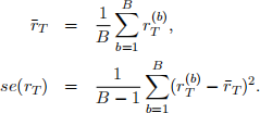
Start an R session, and set a random seed equal to the last 3 digits of your student ID.1 Then generate B sample values of rT (name them as r![]() ;r
;r![]() ;:::;r
;:::;r![]() B)), and compute the sample mean and variance of rT as follows:
B)), and compute the sample mean and variance of rT as follows:
For the purpose of your simulations, set T = 63, 72 = 0:1, B = 1000.
The Sharpe ratio, deÖned as SR = ![]() ), is a common measure of the risk-return tradeo§. Trading strategies with higher SR are more preferred by investors.
), is a common measure of the risk-return tradeo§. Trading strategies with higher SR are more preferred by investors.
Complete the following table with SR values. Comment on the performance of the trading strategies under di§erent scenarios.
|
o〇 |
o1 |
Alice |
Bob |
Carol |
|
0 |
1 |
|
|
|
|
0:01 |
1 |
|
|
|
|
_0:01 |
1 |
|
|
|
|
0 |
0:9 |
|
|
|
|
0 |
1:1 |
|
|
|
2. [Total: 16 marks] Let M denote the mood of Mimi (h: happy; a: angry), and let W denote the weather (s: sunny; r: rainy). The joint probability distribution of M and W is given in the table below. The row and column sums are displayed in the last column and in the last row, respectively.
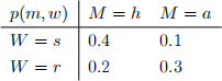
(a) [2 marks] Compute P(M = a).
(b) [2 marks] Derive the conditional distribution of W given M = a.
Assume that, given m and w, your test score S follows a normal distribution with mean 元(m;w) := E(S|M = m;W = w) and standard deviation 5. The conditional mean function
元(m;w) is given in the table below:
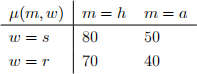
The passing score is 50 or above.
(c) [3 marks] Compute the mean score E(S).
(d) [3 marks] Given that Mimi was angry, what is the mean score you would get? (e) [3 marks] Compute the probability of failing the test.
(f) [3 marks] Given that you failed the test, what is the probability that Mimi was angry?
3. [Total: 20 marks]
Note: Please append your R codes (as a separate .R file) while you submit the assignment.
Carol, an amateur economist, proposes the following time series model for unemployment
rate:
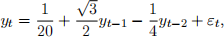 (2)
(2)
where "t ~ iid N(0; 0:022) (normal distribution with mean 0 and variance 0:022). The time period is measured in number of quarters.
(a) [3 marks] Show that the time series {yt} generated by model (1) is stationary.
(b) [3 marks] There is a stochastic cycle in the time series generated by model (1). Find its periodity in number of quarters.
(c) [4 marks] Compute the ACF for the first 3 lags, i.e., o(1), o(2) and o(3).
(d) [2 marks] Write an R program to simulate a sample path of {yt} over 30 years. Set the initial values y〇 and y━1 to be y〇 = 0:1 and y━1 = 0:12. While simulating the random numbers for "t, set the random seed to be your last 3 digits of your student ID.
(e) [2 marks] Plot the sample ACF and record its value for the Örst 3 lags (the values can be retrieved from the acf command output stored as a list). Why are they di§erent from your answers in part (c)?
(f) [3 marks] Using the simulated sample path in part (d), estimate an AR(2) model using the R command arima. Write down the estimated model with the parameter estimates and their standard error. Also record the estimated variance of the innovations. [Important note: the ìinterceptîestimate in the arima output is in fact the unconditional mean; see Rob Hyndmanís page for details: https://robjhyndman.com/hyndsight/ arimaconstants/.]
(g) [3 marks] Using the simulated sample path in part (d) and the R package forecast, plot the point forecast and the conÖdence interval for each period over the next 5 years. Describe the short-run and long-run behaviour of the point forecast and the confidence interval.
2023-03-11