ACCT3011 Big Data Analytics Undergraduate Programmes 2022/23
Hello, dear friend, you can consult us at any time if you have any questions, add WeChat: daixieit
ACCT3011
Big Data Analytics
Undergraduate Programmes 2022/23
SUMMATIVE ASSIGNMENT
Programming Assignment 3: Support Vector Machines
Introduction
In this exercise, you will complete the algorithm for support vector machines (SVMs).
To get started with the exercise, you will need to download the starter code and unzip its contents to the directory where you wish to complete the exercise. If needed, use the cd command in Octave/Matlab or Python to change to this directory before starting this exercise.
Files included in this exercise
. ex1.m – Octave/Matlab script that will help step you through the exercise . ex1.py – Octave/Matlab script for the later parts of the exercise
. ex1data1.mat - Example Dataset 1
. ex1data2.mat - Example Dataset 2
. ex1data3.mat - Example Dataset 3
. svmTrain.m - SVM training function
. svmPredict.m - SVM prediction function
. plotData.m - Plot 2D data
. visualizeBoundaryLinear.m - Plot linear boundary
. visualizeBoundary.m - Plot non-linear boundary
. linearKernel.m - Linear kernel for SVM
. dataset3Params.m - Parameters to use for Dataset 3
. [*] gaussianKernel.m - Gaussian kernel for SVM
* indicates files you will need to complete.
Throughout the exercise, you will be using the scripts ex1.m and/or ex1.py. These scripts set up the dataset for the problems and make calls to functions that you will write. You are only required to modify functions by following the instructions in this assignment.
1 Support Vector Machines
In this exercise, you will be using support vector machines (SVMs) with various example 2D datasets. Experimenting with these datasets will help you gain an intuition of how SVMs work and how to use a Gaussian kernel with SVMs.
The code provided in ex1.m and ex1.py will guide you through the exercise
1.1 Example Dataset 1
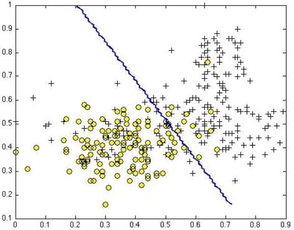
We will begin by with a 2D example dataset which can be separated by a linear boundary. The code in ex1.m and ex1.py will plot the training data (Figure 1). In this dataset, the positions of the positive examples (indicated with +) and the negative examples (indicated with o) suggest a natural separation indicated by the gap. However, notice that there is an outlier positive example + on the far left at about (0.1, 4.1). As part of this exercise, you will also see how this outlier affects the SVM decision boundary.
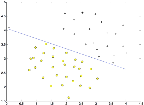
Figure 1: Examples Dataset 1
In this part of the exercise, you will try using different values of the C parameter with SVMs. Informally, the C parameter is a positive value that controls the penalty for misclassified training examples. A large C parameter tells the SVM to try to classify all the examples correctly. C plays a role similar to 1/ λ, where λ is the regularization parameter that we were using previously for logistic regression.
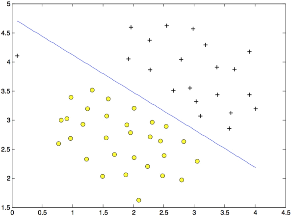
Figure 2: SVM Decision Boundary with C = 1 (Example Dataset 1)

Figure 3: SVM Decision Boundary with C = 100 (Example Dataset 1)
The next part in ex1.m will run the SVM training (with C = 1) using SVM software that we have included with the starter code in svmTrain. When C = 1, you should find that the SVM puts the decision boundary in the gap between the two datasets and misclassifies the data point on the far left (Figure 2).
Your task is to try different values of C on this dataset. Specifically, you should change the value of C in the script to C = 100 and run the SVM training again. When C = 100, you should find that the SVM now classifies every single example correctly, but has a decision boundary that does not appear to be a natural fit for the data (Figure 3).
1.2 Implementation
In this part of the exercise, you will be using SVMs to do non-linear classification. In particular, you will be using SVMs with Gaussian kernels on datasets that are not linearly separable.
1.2.1 Gaussian Kernel
To find non-linear decision boundaries with the SVM, we need to first implement a Gaussian kernel. You can think of the Gaussian kernel as a similarity function that measures the “distance” between a pair of examples, (x(i), x(j)). The Gaussian kernel is also parameterized by a bandwidth parameter, σ, which determines how fast the similarity metric decreases (to 0) as the examples are further apart.
You should now complete the gaussianKernel function to compute the Gaussian kernel between two examples, (x(i), x(j)). The Gaussian kernel function is defined as:
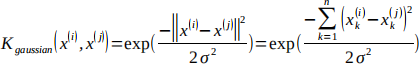
Once you’ve completed the function gaussianKernel, the scripts will test your kernel function on two provided examples and you should see 0.324652.
1.2.2 Example Dataset 2
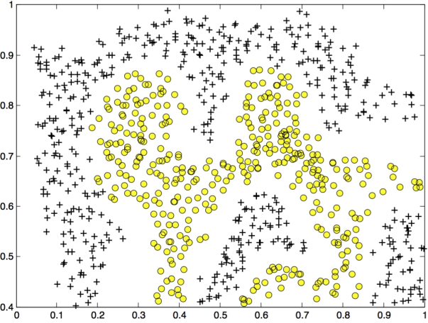
Figure 4: Examples Dataset 2
The next part in ex1.m and ex1.py will load and plot dataset 2 (Figure 4). From the figure, you can observe that there is no linear decision boundary that separates the positive and negative examples for this dataset. However, by using the Gaussian kernel with the SVM, you will be able to learn a non-linear decision boundary that can perform reasonably well for the dataset. If you have correctly implemented the Gaussian kernel function, ex1.m and ex1.py will proceed to train the SVM with the Gaussian kernel on this dataset.
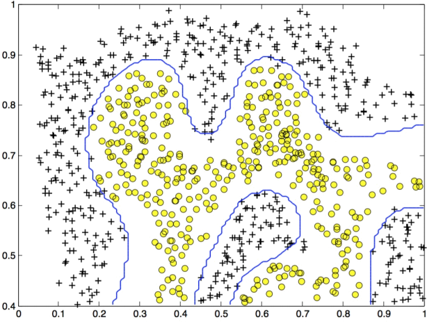
Figure 5: SVM (Gaussian Kernel) Decision Boundary (Example Dataset 2)
Figure 5 shows the decision boundary found by the SVM with a Gaussian kernel. The decision boundary is able to separate most of the positive and negative examples correctly and follows the contours of the dataset well.
1.2.3 Example Dataset 3
In this part of the exercise, you will gain more practical skills on how to use a SVM with a Gaussian kernel. The next part the scripts will load and display a third dataset (Figure 6). You will be using the SVM with the Gaussian kernel with this dataset.
In the provided dataset, ex1data3.mat, you are given the variables X, y, Xval, yval. The provided code in ex1.m and ex1.py trains the SVM classifier using the training set (X, y) using parameters loaded from the function dataset3Params.
You will next use the cross validation set Xval, yval to determine the best C and σ parameter. You should examine the code necessary to search over the parameters C and σ . For both C and σ, you will try values in multiplicative steps (e.g., 0.01, 0.03, 0.1, 0.3, 1, 3, 10, 30). Note that you will try all possible pairs of values for C and σ (e.g., C = 0.3 and σ = 0.1). For example, if you try each of the 8 values listed above for C and for σ2, you would end up training and evaluating (on the cross validation set) a total of 82 = 64 different models.
After you have determined the best C and σ parameters, the code in ex1.m and ex1.py will return a decision boundary shown in Figure 7.
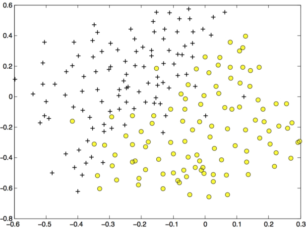
Figure 6: Examples Dataset 3
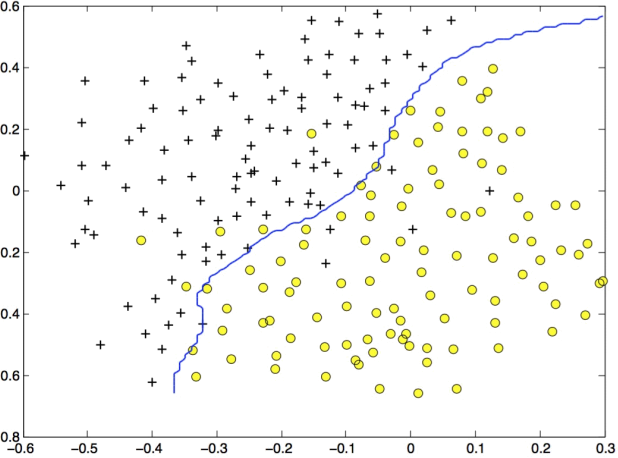
Figure 7: SVM (Gaussian Kernel) Decision Boundary (Example Dataset 3)
Required:
a) Using your own words, briefly define the function gaussianKernel.
b) Create a flowchart solution for gaussianKernel.
c) The SVM solves minθ C ![]() y( i) cost1 (θT x(i))+(1 − y¿¿(i))cost0 (θT x( i))+
y( i) cost1 (θT x(i))+(1 − y¿¿(i))cost0 (θT x( i))+![]() θ j(2)¿ , where the cost functions appear as shown below:
θ j(2)¿ , where the cost functions appear as shown below:
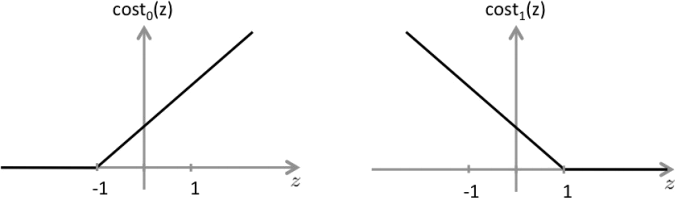
The first term in the objective is: C ![]() y( i) cost 1 (θT x(i))+(1 −y¿¿(i))cost0 ( θT x(i)) . ¿ Identify
y( i) cost 1 (θT x(i))+(1 −y¿¿(i))cost0 ( θT x(i)) . ¿ Identify
and discuss the two conditions that would guarantee that this term equals zero. Suppose you have trained an SVM classifier with a Gaussian kernel, and it learned the following decision boundary on the training set:
You suspect that the SVM is underfitting your dataset. Discuss whether you should try increasing or decreasing C and/or increasing or decreasing σ 2 .
Overall word limit: 500 words
2023-03-03