ACCT3011 Big Data Analytics Undergraduate Programmes 2022/23
Hello, dear friend, you can consult us at any time if you have any questions, add WeChat: daixieit
ACCT3011
Big Data Analytics
Undergraduate Programmes 2022/23
SUMMATIVE ASSIGNMENT
Programming Assignment 2: Neural Networks
Introduction
In this exercise, you will complete the algorithm for neural networks and apply it to the task of hand-written digit recognition.
To get started with the exercise, you will need to download the starter code and unzip its contents to the directory where you wish to complete the exercise. If needed, use the cd command in Octave/Matlab or Python to change to this directory before starting this exercise.
Files included in this exercise
. ex1.m - Octave script that will help step you through the exercise
. ex1.py - Octave script for the later parts of the exercise
. ex1data1.mat - Training set of hand-written digits
. ex1weights.mat - Neural network parameters
. displayData.m - Function to help visualize the dataset
. fmincg.m - Function minimization routine (similar to fminunc)
. sigmoid.m - Sigmoid function
. computeNumericalGradient.m - Numerically compute gradients
. debugInitializeWeights.m - Function for initializing weights
. randInitializeWeights.m - Randomly initialize weights
. nnCostFunction.m - Neural network cost function
. predict.m - Neural network prediction function
. [*] sigmoidGradient.m - Compute the gradient of the sigmoid function * indicates files you will need to complete.
Throughout the exercise, you will be using the scripts ex1.m and/or ex1.py. These scripts set up the dataset for the problems and make calls to functions that you will write. You are only required to modify functions by following the instructions.
1 Neural Networks
In this exercise, you will implement a neural network and used it to predict handwritten digits. In addition, you will complete code in order to implement the backpropagation algorithm to learn the parameters for the neural network. The code provided in ex1.m and ex1.py will guide you through the exercise
1.1 Visualizing the data
Before starting to implement any learning algorithm, it is always good to visualize the data if possible. In the first part of ex1.m, and ex1.py the code will load the data and display it on a 2-dimensional plot by calling the function plotData.
In the first part of ex1.m and ex1.py the code will load and display the data on a 2- dimensional plot (see below Figure 1), by calling the function displayData.
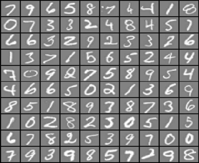
Figure 1: Examples from the dataset
1.2 Implementation
Our neural network is shown in Figure 2. It has 3 layers – an input layer, a hidden layer and an output layer. Recall that our inputs are pixel values of digit images. Since the images are of size 20 × 20, this gives us 400 input layer units (not counting the extra bias unit which always outputs +1). The training data will be loaded into the variables X and y by the ex1.m and ex1.py scripts.
You have been provided with a set of network parameters (Θ (1), Θ(2)) that have been already trained. These are stored in ex1weights.mat and will be loaded by ex1.m and/or ex1.py into Theta1 and Theta2. The parameters have dimensions that are sized for a neural network with 25 units in the second layer and 10 output units (corresponding to the 10 digit classes).
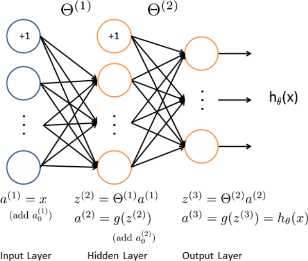
Figure 2: Neural Network Model
2 Backpropagation
In this part of the exercise, you will complete the needed code to run the backpropagation algorithm for the neural networks. You will first use the backpropagation algorithm to compute the gradients for the parameters for the (unregularized and regularized) neural network.
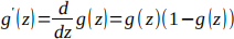
2.1 Sigmoid gradient
To complete this part of the exercise you will need to implement the sigmoid gradient function. The gradient for the sigmoid function can be computed as;
 (1)
(1)
where,
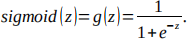 (2)
(2)
When you are done, try testing a few values by calling sigmoidGradient(z) at the Octave/Matlab or Python command line. For large values (both positive and negative) of z, the gradient should be close to 0. When z = 0, the gradient should be exactly 0.25. Your code should also work with vectors and matrices. For a matrix, your function should perform the sigmoid gradient function on every element.
2.2 Backpropagation
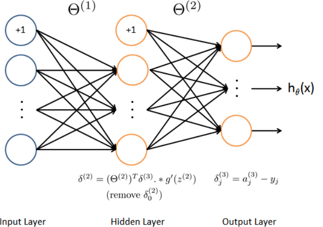
Figure 3: Backpropagation
Now your code will run the backpropagation algorithm as depicted in Figure 3. Recall that the intuition behind the backpropagation algorithm is as follows. Given a training example (x(t), y(t)), we will first run a “forward pass” to compute all the activations throughout the network, including the output value of the hypothesis hΘ (x). Then, for each node j in layer l, we would like to compute an “error term” δ (l) that measures how much that node was “responsible” j for any errors in our output. For an output node, we can directly measure the difference between the network’s activation and the true target value, and use that to define δj(3)(since layer 3 is the output layer). For the hidden units, you will compute δ (l) based on a weighted average of the error terms of the nodes in layer (l + 1).
3 Visualizing the hidden layer
One way to understand what your neural network is learning is to visualize what the representations captured by the hidden units. Informally, given a particular hidden unit, one way to visualize what it computes is to find an input x that will cause it to activate (that is, to have an activation value (a(l)) close to 1). For the neural network you trained, notice that the ith row i of Θ(1) is a 401-dimensional vector that represents the parameter for the ith hidden unit. If we discard the bias term, we get a 400 dimensional vector that represents the weights from each input pixel to the hidden unit.
Thus, one way to visualize the “representation” captured by the hidden unit is to reshape this 400 dimensional vector into a 20 × 20 image and display it. The next step of ex1.m and ex1.py does this by using the displayData function and it will show you an image (similar to Figure 4 below) with 25 units, each corresponding to one hidden unit in the network.
In your trained network, you should find that the hidden units correspond roughly to detectors that look for strokes and other patterns in the input.
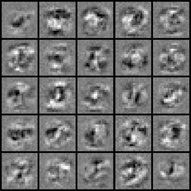
Figure 4: Visualization of Hidden Units.
Required:
a) Using your own words, briefly define the function sigmoidGradient.
b) Create a flowchart solution for sigmoidGradient.
c) Suppose you have trained an ANN, you suspect that the ANN is overfitting your dataset. Discuss what you should decreasing the overfitting problem.
Overall word limit: 500 words
2023-03-03