ECON8026 Final Exam
Hello, dear friend, you can consult us at any time if you have any questions, add WeChat: daixieit
ECON8026 Final Exam
Instructions: This exam contains three questions. You need to answer all questions to obtain full marks. The total maximum marks fbr the entire exam are 80. The breakdown of marks is as follows: question 1, 20 marks; question 2, 20 marks; question 3, 40 marks.
Question 1. 20 Marks, 4 marks for each sub-question a-e
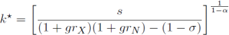
Solow Model The steady-state equilibrium in the Solow model fbr capital per effective worker, k, is:
(1 + g/.x)(i + g’nv) —(1 一 G
where s is the savings rate, a is the elasticity of output with respect to capital, grx is the growth rate of technology, grv is the growth rate of the population, and ◎ is the capital depreciation rate.
Output is produced with a Cobb-Douglas technology, so that output per effective worker is y=ka.
a. ) What is the effect of an increase in the population growth rate on steady-state capital per effective worker and output per effective worker? To answer this, compute the derivates dlnk*/dgrN and dlny*/dgrN.
b. ) What is the effect of an increase in the technology growth rate on steady-state capital per effective worker and output per effective worker? To answer this, compute the derivates dlnk*/dgrx and dlny*/dgrx.
c. ) What is the effect of an increase in the savings rate on steady-state capital per effective worker and output per effective worker? To answer this, compute the derivates dlnk*/ds and dlny*/ds.
d. ) What is the effect of an increase in the elasticity of output with respect to capital on steady-state capital per effective worker and output per effective worker? To answer this, compute the derivates dlnk*/da and dlny*/da.
e. ) What is the effect of an increase in the capital depreciation rate on steady-state capital per effective worker and output per effective worker? To answer this, compute the derivates dlnk*/do and dlny*/do.
Question 2. 20 Marks total, 5 marks for each sub-question a-d
Preference Shocks, Production Shocks, and General Equilibrium. Suppose that firms and consumers co-exist in the static (one-period) consumption-leisure model. The representative firm uses only labor to produce its output good, y, which the representative consumer uses for consumption, c. Suppose the production function is linear in labor, n, so that output of the firm is given by y=An, where A is a production function shock. Suppose there are no taxes of any kind. Firms hire labor in a perfectly competitive labor market.
The consumer's utility function is given by u(Bc, I). The function u satises all the usual properties we assume for utility functions: 6u/6c >0, ^u/Sc2^, 6u/61 >0,锣u/SFvO. B denotes a preference shifter.
a. ) What is the equillibrium real wage in this model?
For each of the following three questions, clearly sketch your answers in one single diagram with consumption on the vertical axis and leisure on the horizontal axis.
b. ) Suppose currently A = Ao and B = Bo (that is, Ao and Bo are some current values for the production shock and preference shock, respectively). On your diagram, clearly (qualitatively) sketch an indifference map, a budget constraint, and associated optimal choices of consumption and leisure.
c. ) Suppose a negative technology shock occurs, lowering,from Ao to A\ < Ao.
B remains the same, that is Bo = B,. On your diagram, clearly sketch an indifference map, a budget constraint, and associated optimal choices of consumption and leisure. Explain any differences between your sketch here and that in part b.
d. ) Suppose a preference shock occurs, lowering B from B from Bo to B, < Bo. . The level of productivity remains unchanged (A, =A0). In your diagram, clearly sketch an indifference map, a budget constraint, and associated optimal choices of consumption and leisure. Explain any differences between your sketch here and those in part b.
Sticky Prices, Price Indexation, and Optimal Long-Run Inflation Targets. Con sider a variation of the Rotemberg model of nominal rigidities. Suppose that the price adjustment cost that wholesale firm i must pay is given by
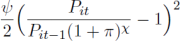
with parameters 寸 2 0 and x NIf X = °, this is exactly the Rotemberg model we have been studying. However, if x > 0, then the adjustment cost is mitigated, and it is only price adjustments that are faster (or slower) than some “normal” rate of inflation tt that incur ("customer anger" and other) costs. Formally, think of tv (without a time subscript) as the steady state (i.e, long-run) rate of price inflation.
As in our basic Rotemberg framework, the adjustment cost is a firm-wide real cost, independent of how many units of output are sold. Hence, the period-i nominal profit function for wholesale firm i is
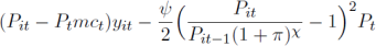
note the Pt term multiplying the adjustment cost term, which converts the real adjustment cost into aggregate nominal units.
The associated period-f resource constraint (in an equilibrium that is symmetric across all wholesale goods firms) in this economy is
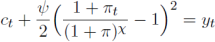
which shows that price adjustment costs are a real resource use in the economy - they drive a gap between total production y and total absorption (here, just c), hence are a deadweight loss.
The rest of the environment is exactly as presented in class: each intermediate firm takes as given its period-^ demand schedule, there is a representative final goods firm that produces final output according to the Dixit-Stiglitz aggregator  , with all the usual notation, etc.
a. Following the setup we developed for the basic Rotemberg framework, construct the dynamic profit-maximization problem of intermediate firm j.
b. Based on the dynamic profit-maximization problem constructed in part a, compute the firm's first-order condition with respect to Pjt.
c. Using the FOC you constructed in part b, impose symmetric equilibrium (i.e., Pt = P/t, Vj, Vf) and then develop an expression in which the only possibly time varying objects are inflation, marginal costs of production, output, and the stochastic discount factor. That is, construct the New Keynesian Phillips Curve (NKPC) for this variant of the Rotemberg model.
d. Consider the deterministic steady state of the expression obtained in part c. Solve for the long-run level of me.
e. If x = 1, which corresponds to the case of full indexation of prices to the long- run inflation rate, how does marginal cost of production compare with the implications of optimal price-setting in the baseline flexible-price Dixit-Stiglitz framework?
2023-02-22