1.

There are 9 variables in the table. The ObservationsC for control group column represents the number of individuals in the control group and Mean1 is the mean value of this variable in the control group. The ObservationsT column represents the number of individuals in the treatment group; Mean2 is the mean value of this variable in the treatment group. The MeanDiff column represents the difference between the means of two groups, and the p-value column is the p-value of the difference.

Table 1 Difference Between the Means of Treatment and Control Groups

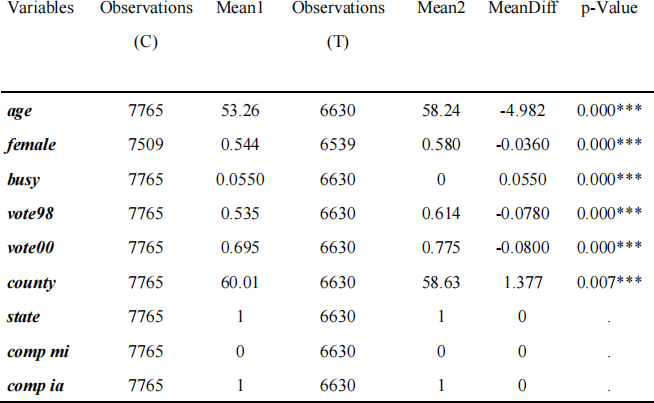
If the value of the variable contact is 1, it means that the individual is in the processing group. Observing the table above, it can be found that there were 6,630 individuals in the treatment group and 7,765 individuals in the control group. The difference in the mean values between the two groups for the first 6 variables was  significant. The remaining 3 variables were the same among individuals in both the treatment and control group.

2.

Since age,female, county, etc., are all variables related to personal traits, there is a gap between the treatment group and the control group, so the potential result of voting cannot only be attributed to the difference between the treatment group and the control group (the variable contact).

3.

The table created in Table 1 and Assignment 1 to test the balance of covariates between the treatment and control groups is similar, but Job 1 The purpose of the table is to verify the randomness of the randomization of individuals to two groups in the first experiment by comparing the mean differences in the means of multiple variables associated with the fixed characteristics of individuals between the treatment and control groups. If it is a random assignment, the values of these specific variables do not differ between the two groups due to processing, so they can be used for proof.

However, Table 1 in this exercise is not related to random grouping. In this experiment, the basis used to distinguish between the control group and the treatment group was whether the participant actually received and listened to the entire call after receiving the call (variable contact). This is not a process of random assignment by the organizers of the experiment, but depends on the participants themselves. Similar  to the variables in the table in Assignment 1, the main explanatory variable in this experiment, contact, was also related to some of the participants' personal traits. Therefore, if you want to add these variables as covariates when doing regression analysis, you need to prove whether there is an autocorrelation between these variables and the variable contact. Then, if these variables differ significantly between the means of the treatment and control groups, then the change in the dependent variable vote02 may be the main explanatory variable or the individual fixed characteristic variable. If so, then the subsequent causal inference cannot be made by  the same way as Assignment 1.

4.

Table 2 Estimated coefficients

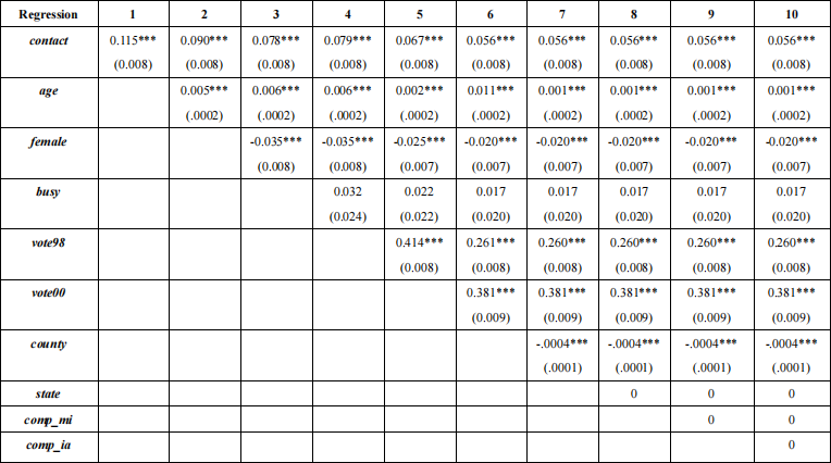
Table 2 above shows the regression coefficients of the independent variables obtained by regression after adding covariates multiple times. For each covariable added to the regression equation, a column was added in Table 2 to represent all the regression coefficients of the new regression equation. Each row corresponds to the regression coefficient of the variable itself in each regression. The parentheses indicate the standard deviation of the regression coefficient for the independent variable. Three asterisks indicate that the independent variable is statistically significant in this regression with a 99% confidence interval. Without an asterisk, the p-value is greater than 0. 1, which means there is no statistical significance at even 90% confidence level.

5.

As can be seen from Table 2, increasing multiple covariates sequentially results in a regression coefficient for the primary explanatory variable, contact, that is, a decrease in the estimate of the treatment effect. But these variables were statistically significant in each regression, except for the variable busy and the three variables of state, comp_mi and comp_ia, which were the same for each subject. From the magnitude of the value of the regression coefficient of the main explanatory variable, contact, the value decreases a little with each additional covariate. This suggests that adding covariates or cancels out estimates of the treatment effect. This shows that the change in the dependent variable vote02 can be explained by the difference between the treatment group and the control group, that is, whether the call is answered and the entire call content is listened to. Throughout the process, some covariates also change the dependent variable. This shows that in this experiment, covariates and treatment together lead to the production of some kind of outcome, or together act as influencing factors.

6.

(a)

In the first assignment, the regression coefficient of the main explanatory variable treat_real, that is, the estimation of the treatment effect, gradually increased with the addition of covariates. On the contrary, as can be seen from Table 2 in this assignment, the regression coefficient of the main explanatory variable contact in this experiment gradually decreases with the addition of covariates.

(b)

In terms of magnitude, the regression coefficient (0.056-0.115) for the variable contact in the results of Table 2 is clearly larger than that of the variable treat_real (about 0.001). In terms of significance, the p-value (0.000) of the regression coefficient of the variable contact is smaller than that of the variable treat_real (0.006).

(c)

One of the main reasons for the differences between the two tables in these respects is that in the regression of Assignment 1, the covariates added to these covariates did not have a significant difference between the mean of the treatment and control groups, but the opposite was true in the regression of this experiment (there was a significant  difference). Therefore, before the regression of Assignment 1, random assignment of participants has been made, as long as a univariate regression with treat_real as the independent variable and vote02 as the dependent variable can be performed and the treatment effect can be estimated properly. Adding covariates is not necessary and interferes with causal inference. However, in Table 2, there is a significant difference  between the two groups of covariates because they are not randomly assigned to 2 groups. Therefore, to use the regression coefficient of the primary explanatory variable contact as an accurate estimate of the treatment effect, several other variables need to be added as control variables. Thus, in the process of multiple regression, the  part of the influence belonging to these covariates has been estimated by their respective regression coefficients, then the regression coefficients of the main variables are accurate estimates of the treatment effect. It can also be seen from the magnitude of the coefficients in the regression results that in Table 2, it is precisely because of the role of the control variables that a more accurate estimated treatment effect can be obtained.

7.

Yes, adding covariates to the regression in Table 2 reduces the bias in the estimation of the treatment effect. As explained earlier, when there is a significant difference between the treatment group and the control group, it is impossible to make accurate causal inference and regression estimation by unary regression, and it is necessary to add covariates as control variables to reduce the bias of estimation. From the change of the regression coefficient of the variable contact in the table, after adding the covariates age,female, vote98 and vote00, the regression coefficient decreased significantly. Among them, the variablefemale minimizes bias. This may be the case because the gender difference itself has the greatest impact on the decision to vote.

8.

No. Because the addition of control variables is only a means of reducing bias, the   above process does not eliminate all bias in the estimate. The possibility of bias also exists in data measurements and statistics, autocorrelation between independent variables, non-measurable or unconsidered interfering variables, and so on.

9. Stata Code

* Open the data set

use "comp_ia_Correction_Last_Name_P_to_Z.dta"

* 1

* Table 1

logout, save(Table2- 1) word replace: ttable3 age female busy vote98 vote00 vote02 county state comp_mi comp_ia , by(contact) pvalue

* 4

* Table 2               reg vote02 contact

reg vote02 contact age

reg vote02 contact age female

reg vote02 contact age female busy